14.6 Fast Fourier Transform
The vast computational task necessary for DFT prevented its practical utilization. In 1965, Cooley and Tukey proposed a computer algorithm that enabled the fast computation of DFT. The algorithm is called Fast Fourier Transform (FFT), has made real-time spectrum analysis a practical tool. In the calculation of the DFT given by equation (14.18), as
![]()
If we were working out values Xn of by a direct approach we should have to make N multiplications of the form ![]() for each of N values of Xn and so the total work of calculating the full sequence Xn would require N2 multiplications. However, the same calculation appears repeatedly since the function
for each of N values of Xn and so the total work of calculating the full sequence Xn would require N2 multiplications. However, the same calculation appears repeatedly since the function ![]() has a periodic characteristic. The FFT algorithm eliminated such repetition and allowed the DFT to be computed with significantly fewer multiplications than direct evaluation of DFT. The FFT reduces this work to a number of operation of the order of 2Nlog2(N) The FFT algorithm has the restriction that the number of data must be 2n(n = 1,2,...,N). This allows certain symmetries to occur reducing the number of calculations (especially multiplications) which have to be done. When the number of data N is N = 2n, DFT needs N2 multiplications and FFT needs 2Nn multiplications, which is only 2n/N of the number of operations. For example, when = 211 = 2048, about 4,194,304 multiplications are necessary in DFT and about 45,056 in FFT, which is only about 1/93rd of number of operations. If N increases this difference increases extremely large. The FFT therefore offers the added bonus of an increase in accuracy. Since fewer operations have to be performed by the computer, round-off errors due to the truncation of products are reduced, and the accuracy increases. If the length of the discrete time series is not equal to 2n(n = 1,2,...,N), then the discrete time series are zero padded (add zeros in the series as discrete data) till it reaches up to the next 2n value. For example, if number of discrete data are 1000, then we need to zero-pad 24 more data to make it to N = 1024 = 210. This will not affect the accuracy of the FFT at all. For example, if we have 520 discrete data then instead of zero-padding 1024-520 = 504 data, the original data may be truncated to next lower value of 29 = 512. This may introduce some error due to truncation of the original data, however, if the discrete time series is long enough then error introduced will be acceptably small. However, the state of the art analog-to-digital equipments now digitizes data 2n(n = 1,2,...,N) in number. For example, the MATLAB (or the SCILAB) has FFT function name fft(xn) where xn = {x}nX1.
has a periodic characteristic. The FFT algorithm eliminated such repetition and allowed the DFT to be computed with significantly fewer multiplications than direct evaluation of DFT. The FFT reduces this work to a number of operation of the order of 2Nlog2(N) The FFT algorithm has the restriction that the number of data must be 2n(n = 1,2,...,N). This allows certain symmetries to occur reducing the number of calculations (especially multiplications) which have to be done. When the number of data N is N = 2n, DFT needs N2 multiplications and FFT needs 2Nn multiplications, which is only 2n/N of the number of operations. For example, when = 211 = 2048, about 4,194,304 multiplications are necessary in DFT and about 45,056 in FFT, which is only about 1/93rd of number of operations. If N increases this difference increases extremely large. The FFT therefore offers the added bonus of an increase in accuracy. Since fewer operations have to be performed by the computer, round-off errors due to the truncation of products are reduced, and the accuracy increases. If the length of the discrete time series is not equal to 2n(n = 1,2,...,N), then the discrete time series are zero padded (add zeros in the series as discrete data) till it reaches up to the next 2n value. For example, if number of discrete data are 1000, then we need to zero-pad 24 more data to make it to N = 1024 = 210. This will not affect the accuracy of the FFT at all. For example, if we have 520 discrete data then instead of zero-padding 1024-520 = 504 data, the original data may be truncated to next lower value of 29 = 512. This may introduce some error due to truncation of the original data, however, if the discrete time series is long enough then error introduced will be acceptably small. However, the state of the art analog-to-digital equipments now digitizes data 2n(n = 1,2,...,N) in number. For example, the MATLAB (or the SCILAB) has FFT function name fft(xn) where xn = {x}nX1.
Example of zero padding/truncation to be included.
16.7 Leakage Error and Countermeasures
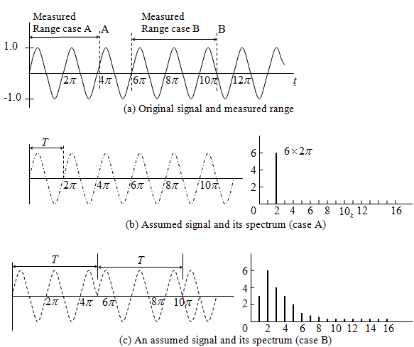
Figure 14.28 The leakage error
In FFT or DFT, computations are based on the assumption that the data sampled over a time period are repeated before and after data measurement. Figure 14.28 shows the assumed signals and their spectra for two types of measurement of a sinusoidal signal x(t) = sint. Both cases have 32 sampled data, but their sampling intervals are different. In case A, the sampling interval is Δt = 4π/32 = 0.3927 and the range measured is exactly twice the fundamental period. The computation of FFT or DFT is performed for the wave as shown by the dotted line (Figure 14.28(b). In this case the assumed wave is same as the original signal and therefore we get a correct signal spectrum. In case B, the sampling interval is Δt = 5π/32 = 0.4909, and the range measured is about 2.5 times the period of the original signal. In this case, the assumed wave shown in Figure 14.28(c) is not smooth at the junction (sometimes discontinuity may occur) and differs from the original signal in time domain. As a result, the magnitude of the correct spectrum decreases and the spectra that do not exist in the original signal appear. As seen in this example, if the time duration measured and the period of the original signal do not coincide, the magnitude of the correct spectrum decreases and spectra that do not exist in the original signal appear on both sides of the correct spectrum. This phenomenon is called the leakage error. It will be illustrated in more detail in the following example.
Example 14.6 Illustrate the leakage error with the help of a simple sine wave. First, take two full-cycles as sampled signal and then take various sampled signals between two full-cycle and two-and-half cycles.
Answer: Figure 14.29(a) show a continuous sine wave of 5 Hz frequency, and its FFT. Figs. 14.29(b-f) shows sampled signal of the continuous sine wave at various time length and corresponding FFT. It can be seen that except 14.29(b) all others have leakage error. The leakage error is seen to increase with the discontinuity at the junction point of the sampled signal for FFT (see 14.29(c-f)). Sufficient points (of the order of 2048) are taken during the sampling and because of that the sampled signal appears as continuous, however, it is discrete points joined by straight lines. At junction point deliberately, the two signals are not joined by a line to show the discontinuity of data more clearly.
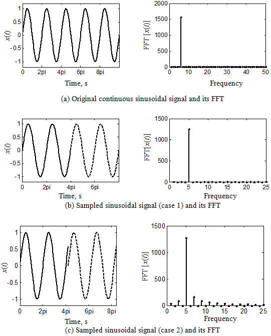
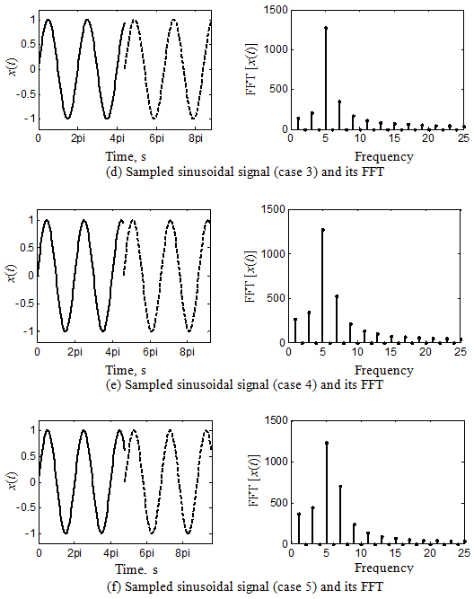
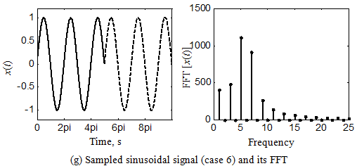
Figure 14.29 A continuous sine wave and its sampled signals with corresponding FFTs
The example illustrate the leakage error with most simple sinusoidal signal. However, the actual measured signal would not be so simple and may contain several frequencies along with randomness. In that case the leakage error is unavoidable; however, the signal processing technique should minimize it. The next section deals with such techniques.
Answer.