Example 14.3 Consider a wave defined as

x(t) = 1 for 0 ≤ t ≤ 1 and 7 ≤ t ≤8
      = 0 for 1 ≤ t ≤ 7

The time period of the wave is T = 8. Obtain the complex Fourier coefficients of the square wave and plot them with respect to gradually increasing Fourier series order (or harmonics) n. It should illustrate how by considering gradual increase in harmonics of the Fourier series, it actually converges to the real signal.

Solution: The given square wave is plotted in Figure 14.18 with its period T = 8.

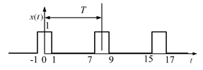
Fig. 14.18 The time history of a square signal

For this square wave, we can obtain complex Fourier coefficients from equation (14.5), as follows

(a)

and

(b)

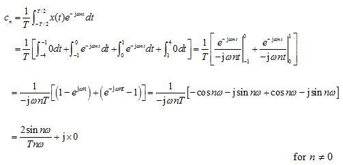
Complex Fourier series coefficients (i.e., the line spectrum) given by equations (a) and (b) are plotted in Figure 14.19 for the real part with respect to n. The abscissa can be taken as frequency (for n = 1, ƒ = 2π/T = 0.784 Hz; similarly for n = k, ƒ = 2π/T = 0.784k Hz;). This diagram is called the spectrum of the time signal. Since given square wave is an even function x(t) = x(-t), imaginary part of c_n  is zero. For an odd function we will have condition as x(t) = -x(-t). These are illustrated in Figure 14.20.

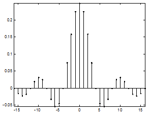
Figure 14.19 (a) The line diagram with actual data of a square wave (complex form)

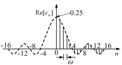
Figure 14.19 (b) The line spectrum and an envelope (dashed line) of a square wave (complex form)

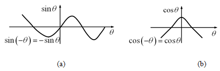
Figure 14.20(a) An odd function (b) An even function

Fig. 14.21 shows a square wave and its various harmonic sine waves, by adding more and more these harmonic waves the square wave could be obtained. Figures 14.22(a)-(g) show how by gradually adding more terms in the Fourier series, it approaches the actual signal. In these figures n represents the number of terms in the Fourier series.

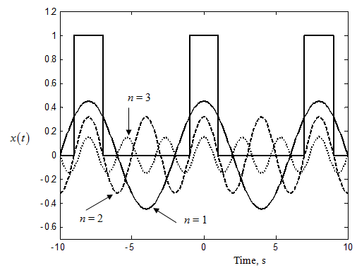
Fig. 14.21 A square wave and its various harmonics

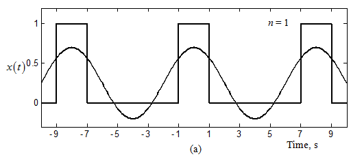
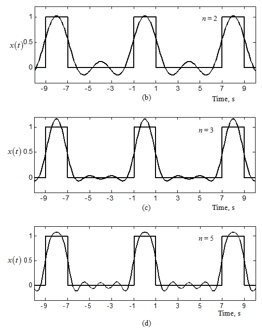
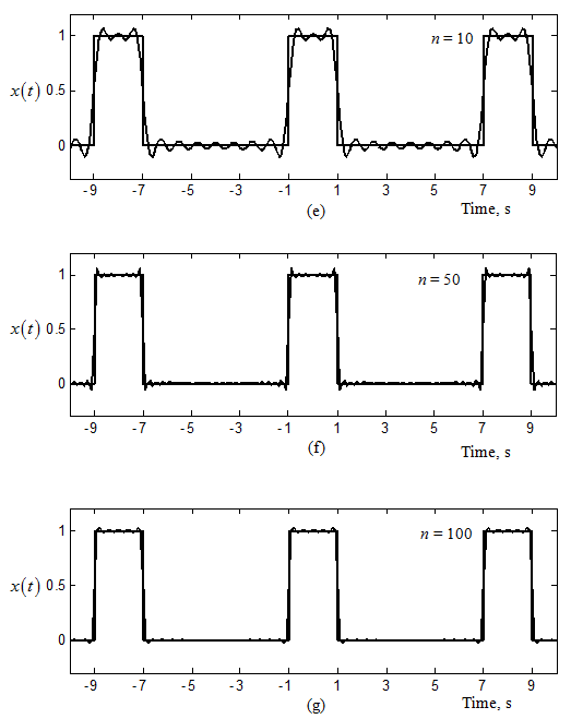
Fig. 14.22 Comparison between the continuous square wave in time domain and the corresponding complex Fourier series up to different harmonics (n is the number of harmonics included)

Answer.