14.5 Discrete Fourier Transform
Till now, we have discussed the Fourier series, Fourier transform and Fourier Integral on the assumption that we know a continuous signal wave (it is also called the continuous time series) in the infinite time domain. However, in practical experiments, the data acquired, converted from the data measured by an analog-to-digital converter, are sequences of data {xn} (n = 0, 1, 2, …, n-1, n) that are discrete and with finite in number. To perform the spectrum analysis using these finite numbers of discrete data (it is also called discrete time series), we must use the discrete Fourier transform (DFT).
In order to estimate spectra from discrete Fourier series the obvious method is to estimate the appropriate correlation function (e.g., the auto- and cross- correlation functions) first, and then to Fourier transform this function to obtain the required spectrum. Until the late 1960s, this was the basis of practical calculation procedures which followed the formal mathematical route by which spectra are defined as Fourier transforms of correlation functions. The assumptions and approximations involved were studied in detail and there is an extensive literature on the classical method (Bendat, et al. 1966). However the position was changed by the advent of the fast Fourier transform (or FFT). This is a remarkably efficient way of calculating the Fourier transform of a discrete time series. Instead of estimating spectra by first determining correlation of a time series and then calculating their Fourier transforms, it is now quicker and more accurate to calculate spectral estimates directly from discrete time series by a method which we shall describe in detail.
This DFT is defined as follows: Given N data sampled with a constant interval Δt, the DFT is defined as a series expansion on the assumption that the original signal is a periodic function with the period NΔt (although the original signal is not necessary periodic). However, various problems occur in the course of this processing. On performing FT in a discrete environment introduces artificial effects, like aliasing effects, spectral leakages, scalloping losses, etc.
If the sampling rate, in the time domain, is lower than the Nyquist rate the aliasing occurs. Two signals are said to alias if the difference of their frequencies falls in the frequency range of interest, which is always generated in the process of sampling (aliasing is not always bad; it is called mixing or heterodyning in analog electronics, and is commonly used in tuning radios and TV channels). It should be noted that, although obeying the Nyquist sampling criterion is sufficient to avoid aliasing, it does not give high quality display in time domain record. If a sinusoid existing in the time signal not bin-centered (i.e., if its frequency is not equal to any of the frequency samples) in the frequency domain spectral leakage occurs. In addition, there is a reduction in coherent gain if the frequency of the sinusoid differs in value from the frequency samples, which is termed scalloping loss.
(a) The first is the aliasing problem. When the signal is sampled with a interval Δt, the information about the components with frequencies higher than ![]() is lost, which is the Nyquist frequency. Therefore, we must only consider to the valid range of the spectra obtained, i.e., below the Nyquist frequency.
is lost, which is the Nyquist frequency. Therefore, we must only consider to the valid range of the spectra obtained, i.e., below the Nyquist frequency.
(b) The second is the challenge of the coincidence of periods. It is impossible to know the correct period of the original signal before the measurement. Therefore, the period of the original signal and the period of DFT do not coincide, and this difference produces the leakage error. We will discuss this leakage error and its countermeasure subsequently (e.g., by window functions).
(c) The third is the problem about the length of measurement. In the case of an isolated signal x(t), we cannot have data in an infinite time range. However, since the Fourier coefficients cn and Fourier transform X(ω) coincide at discrete points as explained in previous section, we can obtain X(ω) by connecting the values of cn smoothly.
Now the procedure of computing the DFT is explained now as follows. Let us assume that we obtained discrete time series x0,x1,x2,x3,....,xN-1 by the sampling. These data are extended periodically to make a virtual periodic signal, as shown by the dashed curve in Figure 14.24.
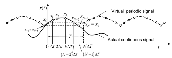
Figure 14.24 Formation of virtual continuous period signal with sampled signal sequences
The fundamental period is T = NΔt and the fundamental frequency is ω0 = Δω = 2π/T. If this dashed curve is given as a continuous time function, its Fourier series expansion is given by the expressions obtained by replacing ω with Δω in equations (14.3) and (14.5). However, in the case of a discrete signal, the integral of equation (14.5) must be calculated by replacing t, T, x(t) and ∫ with kΔt, NΔt, xk and ∑, respectively. By such replacements, we have
|
(14.13) |
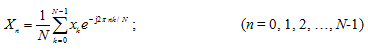
We represent the right-hand side of this expression by Xn, that is
|
(14.14) |
and it is called the discrete Fourier transform of the discrete time signal x0,x1,....,xN-1. Paired with this is the following expression, called the inverse discrete Fourier transform (IDFT)
|
(14.15) |
These transformations map the discrete signal of a finite number on the time axis to the discrete spectra of a finite number on the frequency axis, or vice versa. These expressions using complex numbers are called the complex discrete Fourier transform and the complex inverse discrete Fourier transform. We also have transformation using only real numbers. One is the real discrete Fourier transform, given by
|
(14.16) |
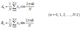
where An and Bn are quantities defined by Xn = An + jBn. Further, the inverse real discrete Fourier transform is given by
|
(14.17) |
We will explain the characteristics of the spectra obtain by the DFT using an example subsequently. Before that let us examine the aliasing effect on the DFT. We have seen that the DFT of the series x0,x1,....,xN-1 is defined by
|
(14.18) |
Suppose we try to calculate values of Xn for the case when n is greater than (N-1). Let for example, n = N + 1. Then,
|
(14.19) |