14.4 Fourier Transform and Fourier Integral

In previous section, we have seen the spacing between adjacent harmonics is Δω = 2π/T and it will be seen that, when the period T becomes large, the frequency spacing  becomes smaller, and the Fourier components become correspondingly tightly packed in Figure 14.19. In the limit when T → ∞, they will in fact actually merge together and the envelope becomes continuous. Since in this case x(t) no longer represents a periodic phenomenon we can then no longer analyse it into discrete frequency components. For example, when x(t) is an isolated pulse, it cannot be converted to a discrete spectrum since it is not periodic. Subject to certain conditions, we can however still follow the same line of thought except that the Fourier series (14.1) (or (14.3)) turns into a Fourier integral and the Fourier coefficients (14.2) (or (14.5)) turn into continuous functions of frequency called Fourier Transforms. Let us consider that this interval is extended to infinity. Then the spectra obtained will represent the spectra of the isolated pulse. On substituting equation (14.5) into equation (14.3), we get

(14.8)

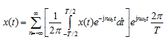
where the frequency ω = 2π/T of the fundamental wave is denoted by ω₀ and is called fundamental harmonics. Here we represent the n^th order by nω₀ = ω_n  and the difference in frequencies between the adjacent components by ω_n+1 - ω_n = ω₀ = 2π/T = Δω. If we make T → ∞, we have

(14.9)

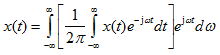
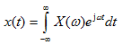
where ω_n, Δω and ∑ are replaced by ω, dω and ∫, respectively. This can be expressed in separate forms as follows

(14.10)

and

(14.11)

Equation (14.11) is called the Fourier transform of x(t) and equation (14.10) is called the inverse Fourier transform (or the Fourier integral) of X(ω). The classical Fourier analysis theory (Churchill, 1941) considers the conditions that x(t) must satisfy equations (14.10) and (14.11) to be true. For engineering applications, the important condition is usually expressed in the form

(14.12)

It means that classical theory applies only to functions which decay to zero when . This condition may be relaxed when impulse functions are introduced in the generalized theory of Fourier analysis. As for the discrete Fourier series, when there is a discontinuity in x(t), equation (14.10) gives average value of x(t) at the discontinuity.

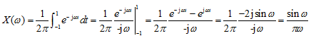
Example 14.4 Consider a square pulse defined as

x(t) = 1 for -1 ≤ t ≤1
      = 0 for all other t

Obtain the continuous spectrum for the pulse and compare the same with the square wave of Example 14.3.

Solution: Figure 14.23(a) shows the square pulse given in the problem. From equation (14.11), i.e., by the Fourier transformation, we get

(a)

Now, let us compare the line spectrum of a square wave of period T as shown in Figure 14.19 and that of a square pulse shown in Figure 14.23(b) in the form of a continuous spectrum. From equation (b) of Example 14.3, we have the Fourier coefficients, C_nas

(b)

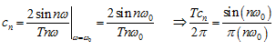
On comparing equation (b) with equation (a) for ω = ω₀, the Fourier coefficients, c_n, and the Fourier transform, X(ω), can be related as

(c)

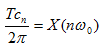
where ω₀ is the fundamental frequency. Therefore, the envelope of the quantities obtained by multiplying T/2π to the line spectra of the Fourier coefficients, c_n, of the square wave gives the continuous spectra of the Fourier transform X(ω) of the square pulse. For example at ω = 0 from equation (a), we have

(d)

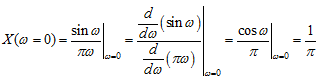
From equation (a) of Example 14.3, we have c₀ = 0.25. Hence, , which is same as equation (d). Similarly, at any other harmonics it can be verified that the Fourier coefficients, c_n, and the Fourier transform X(ω) are related as in equation (c).

(a) Square pulse in time domain	(b) Fourier transform of the square pulse

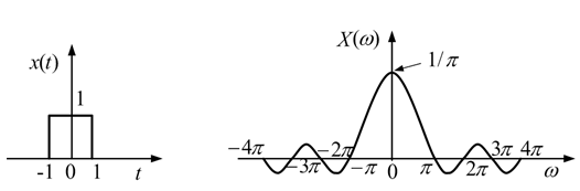
Figure 14.23 A square pulse and its continuous spectrum

Answer.