Example 14.2 The flashing frequency of an stroboscope 30 Hz, what will be the speed of shaft which will appear to the observer when the actual shaft speed is (i) 30 Hz (ii) 60 Hz (iii) 25 Hz (iv) 34 Hz (v) 54 Hz, (vi) 76 Hz and (vii) 600 Hz (viii) 15 Hz and (ix) 45 Hz (x) 13 Hz and (xi) 18 Hz. Give a plot of such variation for each of these cases.

Solution: The following speed of the shaft will be observed (i) stationary 1×30, (ii) stationary 2×30,  (iii) 25 – 30 = - 5 Hz in the opposite direction as the actual shaft rotation, (iv) 34 – 30 = 4 Hz in the same direction as the actual shaft rotation, (v) 54 - 2×30 =- 6 Hz in the opposite direction as the actual shaft rotation, (vi)76 – 2×30 = 16 Hz or 76- 3×30 =- 14 Hz; we will see the minimum of these two, i.e. 14 Hz in the opposite direction as the actual shaft rotation,  (vii) stationary 20×30, (viii) 15 -30=-15 Hz, since it is half the frequency of the shaft if we mark two different colours on the diagonally opposite on the shaft surface we will see them alternatively, (ix) 45-30 = 15 Hz, in this also case if we mark two different colours on the diagonally opposite we will see them in alternatively, (x) 13- 30 =- 17 Hz in the opposite direction as the actual shaft rotation, and (xi) 18 -30 = -12 Hz, in the opposite direction as the actual shaft rotation.

In general if  is the shaft frequency and  is the frequency of the stroboscope then
(a) the Nyquist frequency would be
(b) when  then the shaft will appear as if it is rotating at frequency of  and the virtual rotation of the shaft will be in the opposite to the actual rotation. However, when  if we mark two different colours on the diagonally opposite side of shaft surface, we will see them in alternatively.
(c) when  the shaft will appear as stationary.
(d) when  the shaft will appear to rotate at frequency  in the same direction as the actual.
(e) when  if we mark two different colours on the diagonally opposite we will see them in alternatively.
(f) when  the shaft will appear to rotate at frequency  in the opposite direction as the actual.
(g) when  the shaft will again appear as stationary.
(h) In general, when the shaft will appear as stationary and  if we mark two different colours on the diagonally opposite we will see them in alternatively. When  the shaft will appear to rotate at frequency  in the same direction as the actual. When the shaft will appear to rotate at frequency  in the opposite direction as the actual.

16.3 Fourier Series

In mathematics, a Fourier series decomposes a periodic function into a sum of simple oscillating functions, namely sines and cosines. The study of Fourier series is a branch of Fourier analysis. Fourier series were introduced by Joseph Fourier (1768–1830) for the purpose of solving the heat equation in a metal plate (Fourier, 1822). In data processing, we must first know the frequency components contained in a signal. The fundamental knowledge necessary for it is the Fourier series. We will briefly summaries it from the point of view of signal processing. One type of Fourier series is expressed by real numbers, while the other is by complex number.

(i) Real Fourier Series:

A periodic function x(t) with period T can be expanded by trigonometric functions which belong to the orthogonal function systems as follows (Kreyzig, 2010)

(14.1)

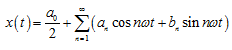
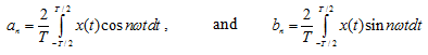
where ω = 2π/T. This series is called the Fourier series or real Fourier series. Its coefficients are given by

(14.2)

The mathematical conditions for the convergence of equation (14.1) are extremely general and cover practically every conceivable engineering situation (Churchill, 1941). The only important restriction is that, when x(t) is discontinuous, the series gives the average value of x(t) at the discontinuity.

(ii) Complex Fourier Series:
Fourier series can be expressed by complex numbers using Euler’s formulas: e^jθ = cosθ + j sinθ  and e^-jθ = cosθ - j sinθ this gives  and . Complex numbers make it easier to treat the expressions. The complex representation also makes it possible to represent a whirling motions of a rotor in two orthogonal planes on the complex plane. Substituting the Euler’s formula into equation (14.1), we have

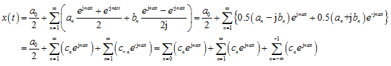
which finally gives

(14.3)

with

(14.4)

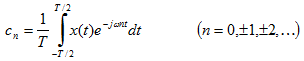
Above expressions give relationship between the real and complex Fourier coefficients, where the complex coefficients are given by

(14.5)

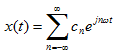
Equation (14.3) is called the complex Fourier series. From equation (14.4), we know the following relationship

(14.6)

which tells that when the real part of complex Fourier coefficients is plotted with respect to the n(n=0,±1,±2,...), it is symmetric about the n = 0. Similarly,  when the imaginary part of complex Fourier coefficients is plotted with respect to the n(n=0,±1,±2,...), it is skew-symmetric about the n = 0. These complex Fourier coefficients can also be represented by

(14.7)

where the absolute value  is called an amplitude spectrum, the angle  a phase spectrum and  a power spectrum.