This phenomenon in which an entirely new signal is obtained during sampling the actual analog (i.e., the continuous) signal, is called the aliasing. This phenomenon could be seen in old movies where the wheel of a horse-cart appears rotating in the opposite direction even when the cart moves forward. This is due to the fact that the rate of picture frame recorded by the camera is much slower than the rotational frequency of the wheel. Another example could be that when we look at an accelerating fan it appears to us in between for some time as if it is rotating in the backward direction (or in the forward direction with very slow speed). It is again due to the fact that the human sight can capture pictures at a certain rate and when the fan speed is just slightly higher than the rate of picture frame captured by the sight, then the fan appears as if it is rotating in opposite direction (or at different speed then it is actually rotating). Similar behaviour is also observed during lightening of cloud while observing the fan in dark. This phenomenon is more obvious when we put stroboscope light on a rotating shaft. In stroboscope the light flashes (switches on and off) at a particular rate, which can be adjustable. When the flashing rate is same as the shaft speed (or integer multiples) the shaft appears as if it is stationary. It due to the fact that whenever light flashes the shaft occupies the same orientation and if we see a mark (or keyway) on the shaft, it will appear stationary. A slight decrease in the flashing rate makes the shaft to appear as rotating slowly in the same direction as the actual direction (when flashing rate is slightly lower than the shaft speed the mark on the shaft will shift in forward direction in the subsequent flashes and hence the shaft will appear as it is rotating in forward direction with slower speed i.e. with a speed equal to the difference between the actual shaft speed and flashing rate), however, a slight increase in the flashing rate makes the shaft to appear as if rotating slowing in backward direction as compared to the actual direction of rotation.
It is obvious that we must sample with a smaller sampling interval as the signal frequency increases. This suggests that aliasing effects not only changes the amplitude and frequency but also the whirl direction of a rotor. We can determine whether or not we have this aliasing by following the sampling theorem. It says: when a signal is composed of the components whose frequencies are all smaller than fc, we must sample it with a frequencies higher than 2fc for the sake of not losing the original signal’s information. The frequency 2fc is called the Nyquist frequency. For example, if a sine wave with period T is sampled whenever x(t) = 0, that is, with sampling interval T/2, we have xn(i.e., a signal with a constant amplitude of zero as shown in Fig. 16.11(b)). Moreover, if it is sampled whenever x(t) = A (where A is the amplitude), that is, with sampling interval T/2, we have xn = A (i.e., a constant amplitude signal). Therefore, two samplings in a period are clearly insufficient. However, this theorem teaches us that digital data with more than two points during one period can express the original signal correctly. Figs. 14.11(c-h) show sampled signal of Fig. 14.11(a0 with sampling frequencies of 17, 20, 24, 30, 40, and 50 Hz, respectively. It can be seen that as the sampling frequency is increased the original signal is getting sampled.
For example, if we sample the signal having components of 1, 2 and 7 kHz with a sampling frequency of 10 kHz. Then 1 and 2 kHz signal will be measured without aliasing effect since the Nyquist frequency is 10/2 = 5 kHz and is more than these vibration signal frequencies. However, we have an imaginary spectrum of 3 kHz (10 kHz - 7 kHz = 3 kHz), which does not exist practically. But, if we sample it with a frequency of more than 14 kHz ( 2 x 7 kHz), such an aliasing problem does not occur. In practical measurements, we do not commonly determine the sampling frequency by trial measurement. Instead, we use a low-pass filter to eliminate the unnecessary high-frequency components in the signal and sample with the frequency higher than twice the cutoff frequency. By such a procedure, we can prevent aliasing.
Example 14.1 If we sample the signal having components of 120, 200, 460, 700, 800 and 900 Hz with a sampling frequency of 1000 Hz. Whether aliasing effect will be present in the measurement? What are the frequencies that will appear in the captured signal?
Solution: The sampling frequency is 1000 Hz, hence the Nyquist frequency will be 1000/2 = 500 Hz. Hence, we can be able to measure frequency below 500 Hz accurately that means frequency 120, 200 and 460 Hz will be measured accurately (Figs. 14.12-16.14). However, frequency 700 Hz will appear as 1000-700 = 300 Hz (Fig. 14.15) and frequency 800 Hz will also appear as 1000-800 = 200 Hz (Fig. 14.16). Frequency 900 Hz will appear as 1000-900 = 100 Hz signal (Fig. 14.17). So the captured signal will contain erroneous high amplitude of 200 Hz signal with an additional frequency of 100 and 300 Hz which is actually not present at all in the actual signal.
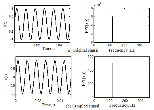
Fig. 14.12 A signal of 120 Hz sampled with sampling frequency 1000 Hz
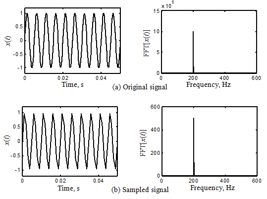
Fig. 14.13 A signal of 200 Hz sampled with sampling frequency1000 Hz
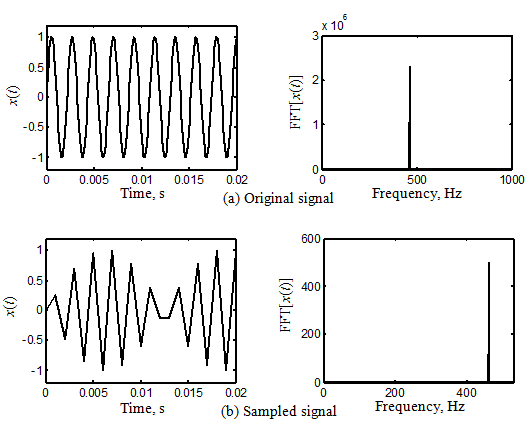
Fig. 14.14 A signal of 460 Hz sampled with sampling frequency1000 Hz
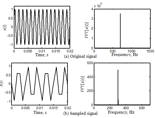
Fig. 14.15 A signal of 700 Hz sampled with sampling frequency1000 Hz
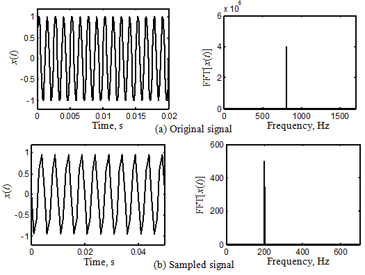
Fig. 14.16 A signal of 800 Hz sampled with sampling frequency1000 Hz
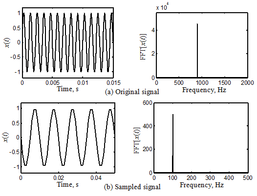
Fig 14.17 A signal of 900 Hz sampled with sampling frequency1000 Hz