(ii) Thirty-two sampled points: The period of the signal is same as 8 sec, hence the fundamental frequency would also be same as f0 = 1/T = 1/8 = 0.125 Hz. The sampling interval is now Δt = T/N = 8/32 = 0.25 sec. The Nyquist frequency would be fc = 1/2ΔT = 1/(2 X 0.25) = 2 Hz. Hence, the maximum harmonics which will be valid is n = fc/f0 = 2/0.125 = 16. Total number of harmonics are same as number of sampled points, i.e., 32.
When the sampling interval is narrowed (from 0.25 sec to 0.125 sec) the number of spectra increases (from 16 to 32) as shown in Figure 14.27, and therefore such a spectra diagram written in the interval Δω = 2π/T(which remains constant since T is constant) extends to the right (from 2 Hz to 4 Hz). An envelope is shown by dashed line of the spectra in Figure 14.27. If the sampling frequency is shortened continuously, the sampled data become substantially equal to the continuous wave, and therefore its spectra will approach those of the Fourier series shown in right half of Figure 14.23(b). The magnitude of X0 is 0.313 in Figure 14.26(a) and X0 is 0.281 in Figure 14.27. This value approaches c0 = 0.25 in Figure 14.23(b) as the number of data sampled increases. Answer.
Different types of definition of DFT and IDFT are used, depending upon personal preference. Some use the following definitions, in which the magnitudes of Xn coincide with that of Fourier transform X(ω) in Figure 14.23(b).
|
(14.26) |
and
|
(14.27) |
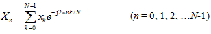
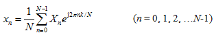
Some use following expressions, which have the coefficient 1/N in the counter-part expression: (MATLAB uses this)
|
(14.28) |
and
|
(14.29) |
Of course, every definition has the same function as mapping from time domain to frequency domain. Especially, when we are interested in the critical frequencies at which amplitudes have peaks, then all the definitions can be used equally well. However, we must be careful when we interpret the physical meaning of the magnitude of the spectra. For example, for x(t) = sin t, it is equation (14.14) that gives a spectrum with magnitude 1.