Equation (u) becomes,
![]()
which gives two natural frequencies of the system for the pure translator motion, as
![]()
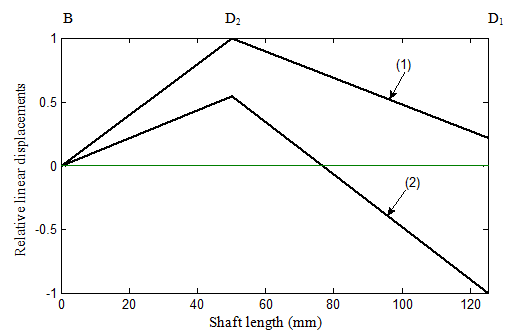
Figure 8.12 Mode shapes; (1) - first mode shape, (2) - second mode shape
The mode shapes corresponding to these natural frequencies are plotted in Fig. 8.12. While plotting mode shapes the maximum displacement corresponding to a particular mode has been chosen as unity and other displacements have been normalized accordingly. Corresponding to the first mode both discs have an in-phase motion, whereas, for the second mode two discs have an anti-phase motion. It should be noted that for the case when discs have appreciable diametral mass moment of inertia, then along with the forces at stations 1 and 2, the moments also need to be considered while deriving influence coefficients. In that case, we will have sixteen influence coefficients, i.e., the size of the influence coefficient matrix would be 4×4, however, the symmetry conditions of influence coefficients will still prevail. Correspondingly, we would have four natural frequencies and corresponding mode shapes. Answer .
Example 8.4 Find transverse natural frequencies and mode shapes of a rotor system as shown in Figure 8.13. B is a fixed bearing, which provides fixed support boundary condition; and D1 , D2 , D3 and D4 are rigid discs. The shaft is made of the steel with the Young's modulus E = 2.1 (10)11 N/m2 and the uniform diameter d = 20 mm. Various shaft lengths are as follows: D1D2 = 50 mm, D2D3 = 50 mm, D3D4 = 50 mm and D4B2 = 150 mm. The mass of discs are: m1 = 4 kg, m2 = 5 kg, m3 = 6 kg and m4 = 7 kg. Consider the shaft as massless and the disc as point masses, i.e., neglect the diametral and polar mass moment of inertia of all discs.
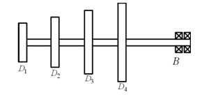
Figure 8.13 A multi-disc cantilever rotor
Solution : The first step would be to obtain influence coefficients. We have the translational deflection, y , and force relations from the strength of material for a cantilever shaft with a concentrated force at any point (Fig. 8.14) as (see Appendix 8.1)
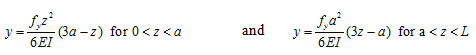 |
(a) |
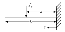
Figure 8.14 A cantilever shaft with a concentrated force at any point
Let us take stations 1, 2, 3, and 4 at each of the disc locations. Figure 8.15 shows a cantilever shaft with forces at stations 1 and 2. Station 1 is at free end and it has an intermediate station 2 between station 1 and the fixed support. Lengths L , l1 , and l2 are shown in Fig. 8.15 and for this case we have L = l1 + l2 . Between two stations, it will have the following influence coefficients (which relates the force to translational transverse displacement from eqn. (a))
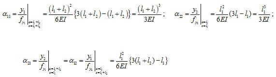 |
(b) |
Similar relations would also be valid between stations (1, 3) and (1, 4), in which values of l1 and l2 would be taken according to the node location (refer Table 8.2 for detail).
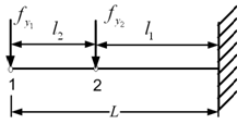
Figure 8.15 A cantilever shaft with a force at the free end and another at the intermediate point