3.2.5 Numerical analysis procedure of finite radial bearings

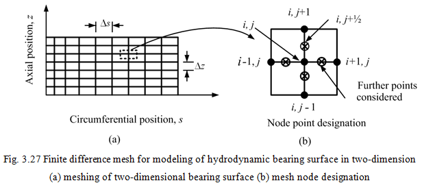
In practice real hydrodynamic bearings cannot be accurately modeled as either the case of infinitely long bearing or the case of infinitely short bearing. Most bearings have a length-to-diameter ratio in the range 0.5 to 1.5. Hence, the approximate solutions of the short or long bearing may be used in preliminary design calculations only. However, final design studies will often require a more realistic analysis by at least using two-dimensional Reynolds equation. For a more general solution of the Reynolds equation, which is a partial differential equation, it is necessary to use numerical methods. The most common numerical technique used in hydrodynamic journal bearing analysis is the finite difference method, because of its relative ease with which it can be adapted to most bearing geometries. The problem is reduced to a two dimensioned by considering the fluid film to be unwrapped from around the journal (Fig. 3.20c). The unwrapped fluid film is then divided into a number of sections of finite size by describing it in terms of mesh nodes, as shown in Figure 3.27a. Here s is the circumferential position and z is the axial position. In between each nodes described, a number of further points are considered, for example those surrounding the node (i, j) are shown in Figure 3.27b. Since the Reynolds equation describes the behavior of the lubricant at any location in the fluid film, it can be written for every specific node contained within the finite-difference mesh.

Equation (3.81) may be written for the node (i, j) as

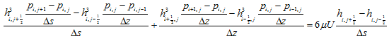(3.85)

which can be rearranged as

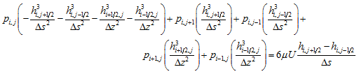(3.86)

and finally which can be simply written as

(3.87)

with

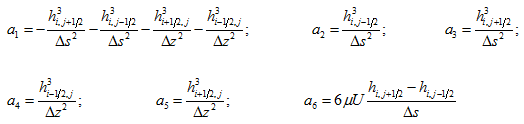
where h_i,j+1/2 is the film thickness between (i, j) and (i,  j + 1) nodes; and a₁, a₂ etc. are constants whose values are known for every nodes. Equation may then be written for every node in the mesh, except for those where the lubricant pressure is already known (for example at the nodes representing the ends of the bearing where the lubricant pressure must be equal to the ambient pressure). These equations can then be solved simultaneously to get lubrication pressure at all nodes.

On estimating the lubricant pressure for a particular journal attitude angle, Φ, and eccentricity, e_r, (i.e., then film thickness will be known), the corresponding forces provided by the lubricant on the journal may be evaluated by summing numerically all of the element forces associated with each node. For example, each node pressure is considered to contribute to force on the journal over an area Δs  & Δz surrounding it as shown in Figure 3.28(a) with shades, when integrating using a trapezium rule.

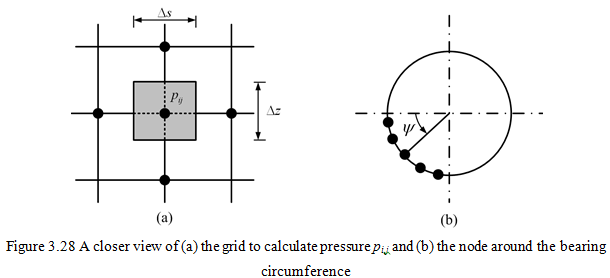
Thus, if the node is situated at some angle ψ to the horizontal direction as shown in Figure 3.28b, then the lubricant force on the journal in the horizontal direction (from left to right) is

(3.88)

and that in the vertical direction (upwards) is

(3.89)

where i is the axial node positions (total n such nodes) and j is the circumferential node position (total m such nodes). For present formulations, lubricant forces acting on the journal should also include the tangential friction forces, however, the friction forces are small when compared with the pressure forces.