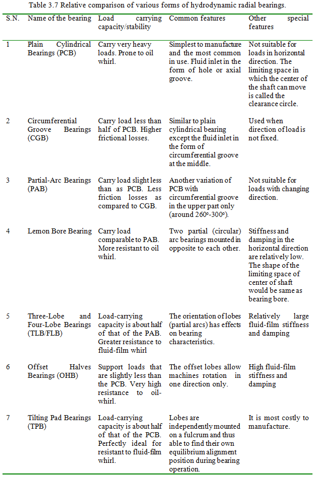
Bearing identification number: Identification numbers of rolling bearings are composed of the basic numbers and the auxiliary codes. The basic numbers are made up of a bearing series symbol, and a dimension series symbol. For example, in bearing basic no. 6204, various numbers representation are as follows: 4 represents diameter series (other options: 8, 9, 0, 1, 2, 3 and 4); 0 represents width series (other options: 1, 2, 3, 4, 5, and 6) and 62 represents bearing series (62 for radial ball bearing, 72 for angular contact ball bearing, 320 for tapered roller bearing, etc.). The auxiliary codes are attached to basic number to identify seal or shield codes, race configuration code, clearance code and tolerance class codes (Harris, 2001).

In rolling element bearings, very high speeds are those speeds having number (is called DN number) more than 3 millions, where d is the bore diameter in mm and N is the bearing operating speed in rpm (for example, for d = 30 mm and N = 1,00,000 rpm or d = 100 mm and N = 30,000 rpm or d = 600 mm and N = 5,000 rpm would give the same DN number of 3 millions). High-speed bearings find applications in aerospace and space technologies. Applications of low speed bearings are (i) gyroscopes: they have very long life of the order of 15 years and they are very high precision bearings. Lubrication for such bearings is quite challenging since it requires about one to two drops per year. Micro and nano-pumps may have very useful applications for such lubrication flow rate; (ii) rotary kiln: it is used in cement factories and have rotational speed of 2 to 3 rpm, however, the size of bore diameter is of the order of 4 m or so.

3.2.2 Reynolds equation and its basic assumptions
It is known from fluid mechanics that a necessary condition for pressure to develop in a thin film of fluid is that the gradient and slope of the velocity profile must vary across the thickness of the film. The analysis of hydrodynamic bearings can be performed theoretically by correctly modeling the bearing fluid film. The assumptions for calculation of performance of the hydrodynamic bearing include:

1. Film thickness is small as compared with journal dimensions.
2. Journal is cylindrical and bearing surface is without local distortion.
3. Journal axis is parallel to bearing axis.
4. Inertia of fluid in film is negligible.
5. Fluid film unable to sustain sub-atmospheric pressure.
6. Fluid pressure is atmospheric in supply, drain and at region where fluid film is broken or cavitated.
7. Laminar flow in the bearing fluid film.
8. Viscous shearing loss in the clearance region outside the pressure field and this space is taken as partly filled with fluid.
9. No frictional losses from the fluid in the groove or drain spaces adjoining journal.
10. Fluid is a simple Newtonian liquid with viscosity independent of the shear rate.
11. The viscosity and density of fluid is constant throughout the bearing.

In real bearings the departures from these assumptions are bound to be there, however, it appears that in bearings for turbomachinery a number of the assumptions are approximately fulfilled, and in many cases the departures from fulfillment of others does not seriously invalidated the overall results of the conventional theory. Departure is likely to be serious when the film-flow is turbulent.

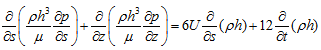
The analysis by which these assumptions are applied in calculation of the dynamic characteristics of the hydrodynamic bearings is only outlined here.  Detailed treatment can be found in (Cameron, 1981; Hamrock, 1994). The governing equation which represents the dynamic behaviour of hydrodynamic bearing was first derived by Reynolds (1886) and is

(3.78)

where s is the distance around the bearing circumference of the point under consideration measured from some arbitrary reference, z is the position of the point under consideration in the axial direction, h(s, t) is the film clearance, p is the lubricant pressure, U is the tangential velocity of the journal surface, ρ is the density of lubricant, µ is the dynamic viscosity of lubricant, and t is the time. The effects of curvature can be ignored for the purposes of evaluation of the lubricant pressure variation since the fluid-film thickness is very small compared with the journal diameter. By doing this we reduce the problem to two-dimensional and for the purpose of mathematical modeling, the lubricant film may be considered as through it were unwrapped from around the journal as indicated in Figure 3.20.

In Figure 3.20, θ is the angular position around the bearing measured from JB produced, Φ is the attitude angle, L is the bearing length, B is the bearing center, J is the journal center, R is the journal radius and  = e is the eccentricity. In most applications the lubricant density does not vary substantially throughout the fluid film. Its viscosity might vary; a constant effective viscosity based on the lubricant thermal balance may be used for calculations. With constant lubricant density and viscosity, the factorρ may be dropped since it is common in all terms, and µ may be taken outside the differential in equation . With basic assumptions mentioned and for the steady-state operation (i.e., ∂h/∂t =0), from equation (3.78) we get

(3.79)

The equation remains applicable with non-circular bore of the bearing.