On either sides of the equilibrium bond length r₀, the PE rises as a symmetric quadratic function (a parabola).  The vibrational wavefunctions can be obtained by solving the Schrodinger equation.  The Hamiltonian operator (for energy) now consists of a kinetic energy term and a potential energy term V as shown in Fig. 13.4 and the solutions for energy, E_v have already been given in Eq.(13.20).  The selection rules for the harmonic oscillator are:

Δv = ± 1                                                                                                                               (13.22)

We will see  several equally spaced lines (spacing hν) corresponding to the transitions 0→1, 1→2,  2→3 and so on.  The first transition will be the most intense as the state with v = 0 is the most populated.

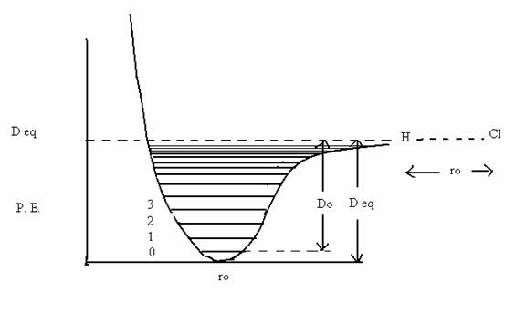
In actual diatomics, the potential is anharmonic.  A good description of an anharmonic oscillator is given by the Morse function.

                                    P.E.  =  D_eq [1 – exp {a(r_o-r }]²                                                           (13.23)

In Eq. (13.22), D_eq is the depth of the PE curve and r₀ is the bond length.  A plot of the Morse curve and the energy levels for the Morse potential are given in Fig. 13.5.  The formula for the energy levels of this anharmonic oscillator is

E_v/hc = e_v  = (v+ ½) ν -  (v+ ½)² ν x_e,  cm^-1                                               (13.24)

Here x_e, is called the anharmonicity constant whose value is near 0.01.  It can be easily deduced from the above formula that the vibrational energy levels for large υ start bunching together.