Ku (1998) developed a C 0 class (i.e., a compatibility requirement of only field variables instead of C 1, in which up to the first derivative of field variables compatibility is required) Timoshenko beam finite element model to study combined effects of shear deformations and the internal damping on the forward and backward whirl frequencies, and onset speeds of the instability threshold of a flexible rotor systems supported on the linear stiffness and damping bearings. Mohiuddin and Kulief (1999) presented a finite element formulation of a rotor bearing system. The model coupled the bending and torsional motions of the rotating shaft and derived by using the Lagrangian approach. The model accounts for gyroscopic effects as well as the inertia coupling between the bending and torsional vibrations. A reduced order model was obtained using model truncation. Model transformations involved the complete mode shapes of a general rotor system with gyroscopic effects and anisotropic bearings. Nelson (1998) gave a comprehensive review of some of the modelling and analysis procedures developed for understanding and simulation of the characteristics of rotor dynamic systems.
The above review gives an idea that there is a vast amount of literatures that are available on the finite element analysis of rotor systems. However, for a beginner it is difficult to follow these literatures. The aim of the subsequent section would be to give a lucid presentation of the finite element formulation of the most simple rotor model, i.e. for the Euler-Bernoulli beam model. In subsequent chapter, the Timoshenko beam model with gyroscopic couple would be dealt.
9.5 A Finite Element Formulation
Vibrating beams are most frequently modelled using the Euler-Bernoulli beam hypothesis. It is because of its simplicity and a well established an accurate prediction to the real motion in the case of relatively thinner beams. Previously, in the present chapter the Euler-Bernoulli beam theory was considered and equations of motion were derived by continuous system approach using the Hamilton's principle. Now, by using the Galerkin method, the finite element formulation and associated consistent mass and stiffness matrices are obtained. For the present case the whirling motion of the beam in the vertical and horizontal directions are uncoupled. The analysis in the vertical plane (i.e., y -z plane) is presented and it will be identical in the horizontal plane (i.e., z-x plane). For obtaining bending natural whirl frequencies, the eigen value problem formulation is presented. Numerical examples are presented for obtaining system natural whirl frequencies, mode shapes and unbalance responses.
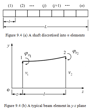
Boundary conditions of a problem are not required while developing the finite element formulation for the shaft. Let us discretise a given shaft into several finite elements (Fig. 9.4a), and consider an element at a distance z in the plane y-z as shown in Figure 9.4b. The length of the element is l . The element has two nodes 1 and 2. Let v be the nodal translational displacement and ![]() be the nodal rotational displacement at any intermediate point of the shaft element, with subscripts 1 and 2 these displacements would belong to respective nodes. The translational and rotational displacements are acting in the positive axis directions at nodal points and are shown in Figure 9.4.
be the nodal rotational displacement at any intermediate point of the shaft element, with subscripts 1 and 2 these displacements would belong to respective nodes. The translational and rotational displacements are acting in the positive axis directions at nodal points and are shown in Figure 9.4.
In the finite element model, continuous displacement variables ![]() are approximated in terms of discretised displacements at nodes of an element
are approximated in terms of discretised displacements at nodes of an element ![]() . Therefore, the displacement can be expressed within the element by using appropriate shape functions, as
. Therefore, the displacement can be expressed within the element by using appropriate shape functions, as
![]()
where ![]() is the row vector of the shape function,
is the row vector of the shape function,![]() is the nodal displacement vector, and superscripts: (e) and (ne) represent an element and nodes of the element , respectively. Let r be the number of nodal displacements on the element, then the number of shape functions would also be equal to r . The explicit form of shape functions and nodal displacement vector would be provided subsequently.
is the nodal displacement vector, and superscripts: (e) and (ne) represent an element and nodes of the element , respectively. Let r be the number of nodal displacements on the element, then the number of shape functions would also be equal to r . The explicit form of shape functions and nodal displacement vector would be provided subsequently.