2.5.1: Calculation of natural frequencies: For obtaining natural frequencies of the system the determinant of the dynamic stiffness matrix, [Z] = ([K] - ω2[M]), should be equated to zero and solved for ω, which gives four natural frequencies of the rotor system. It should be noted that since two orthogonal plane motions are uncoupled (i.e., corresponding to y and φx, and x and φy). hence, equations of motion of each plane could be solved independently This would make the size of [Z] matrix to half. It will be illustrated through examples subsequently. More general method based on the eigen value problem will be discussed in subsequent sections.
2.5.2: Unbalance forced response: The unbalance forcing with frequency, ω, can be written as
(2.82) |
where {Funb} is the complex unbalance force vector and it contains the amplitude and the phase information,k represent row number in vector ![]() and N is the total DOFs of the system (N = 4 for the present case). The response of the system can be written as
and N is the total DOFs of the system (N = 4 for the present case). The response of the system can be written as
(2.83) |
On substituting equations (2.82) and (2.83) into equation (2.81), we get the unbalance response as
(2.84) |
where [Z] is the dynamic stiffness matrix. Similar to the force amplitude vector, the response vector will also have complex quantities and can be written as
(2.85) |
which will give amplitude and phase information, as
(2.86) |
Equation (2.84) is more a general form of the Jeffcott rotor response as that of the disc at mid-span. However, it is expected to provide four critical speeds corresponding to four-DOFs of the rotor system. Most often it is beneficial to observer the amplitude and the phase of response rather than the time history. The present method gives the response in frequency domain. When the damping term is also present, the above unbalance response procedure can easily handle additional damping term, and the dynamic stiffness will take the following form
(2.87) |
where [C] is the damping matrix. It should be noted that [Z] is now a complex matrix and by the numerical simulation critical speeds can be obtained by noticing peaks of responses while varying the spin speed of the shaft. The procedure for obtaining damped natural frequencies will be discussed subsequently. The analysis of the present section is equally valid for other boundary conditions. The only change would be the expressions of influence coefficients corresponding to new boundary conditions (e.g., cantilever, fixed-fixed, free-free, overhang, etc.).
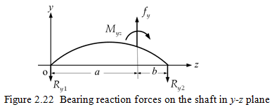
2..5.3: Bearing reaction forces: Bearings are, in the present study, assumed to transmit only forces and not moments. Forces transmitted through bearings are those, which are related to the deflection of the shaft as shown in Figure 2.22 on the y-z plane.
On taking moments about ends L (left) and R (right) of the shaft, we have
(2.88) |
and
(2.89) |
From above equations, bearing reaction forces at the left and right sides are related to the loading on the shaft, fy and Myz. In matrix form equations (2.88) and (2.89) can be written as
(2.90) |
with
![]()
where subscripts: b and s represent the bearing and the shaft, respectively. Complex vectors {Fb} and {Fs} are bearing forces at the shaft ends and shaft reaction forces at the disc, respectively. On using equations (2.79) and (2.84) into the form of equation (2.90) for both plane motions (i.e., y-z and z-x), we get
(2.91) |
with
![]()
It should be noted that equation (2.91) has been written for both plane motions (i.e., y-z and z-x), however they are uncoupled for the present case. Similar to the unbalance force amplitude vector, the bearing force vector will also have complex quantities and can be written as
(2.92) |
where nb is the number of bearing. This will give the amplitude and the phase information, as
(2.93) |
It should be noted that for the case of no damping the phase remains zero between a force in one plane and a response in that plane. These procedures will be illustrated now with simple numerical examples.