14.9.4 Probability Distribution and Probability Distribution Function
Many naturally occurring random vibrations have the Gaussian probability distribution, which is defined as

(14.52)

where m and σ  represent mean and variance, which are constants for a particular random process. Fig. 14.41 is a comparison of the probability density with Gaussian approximation and the actual distribution (without smoothening) from signal in Fig. 14.37. However, Fig. 14.42 shows the comparison of probability density with the Gaussian approximation and the actual distribution (with smoothening).

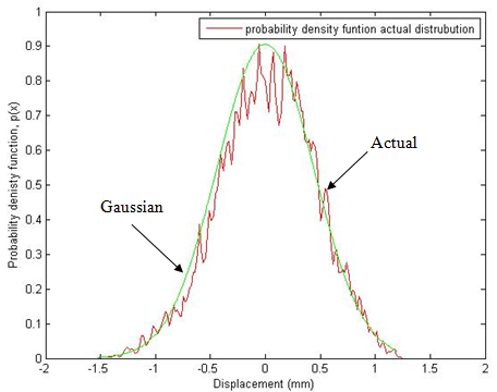
Figure 14.41 Gaussian probability density versus actual probability density without smoothening

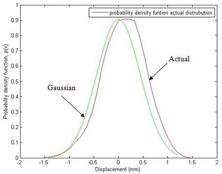
Figure 14.42 Gaussian probability density versus smoothened actual probability density

14.9.5 Ensemble Average, Temporal Average, Mean, Variance

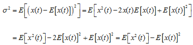
The variance is defined as the mean-square value of the difference from the mean value. Thus

(14.53)

with

and

where E[x²(t)]  is the square-mean and E[x(t)]² is the mean-square. It should be noted that as E[x(t)] is given by the first moment of area of the probability density curve about the p(x) axis (see eqn. (14.44)). So σ² which is given by equation (14.53) and it is the expectation of (x(t) - E[x(t)])², is given by the second moment of area about (x = E[x(t)]), i.e.

(14.54)

σ is the radius of gyration of the probability density curve about (x = E[x(t)]). If the mean value is zero the variance is given by

(14.55)

To evaluate ensemble averages, it is necessary to have information about the probability distribution of the samples or at least a large number of individual samples. Given a single sample x^(j) of duration T it is, however, possible to obtain averages by averaging with respect to time along the sample. Such an average is called a temporal average in contrast to the ensemble or statistical averages described previously. The temporal mean of x(t)

(14.56)

and the temporal mean square is

(14.57)

where the angular brackets represent the temporal average. When x(t) is defined for all time averages are evaluated by considering the limits as T → ∞. For such a function a temporal autocorrelation  can be defined

(14.58)

When  is defined for a finite interval, then similar expression can be used by carefully choosing the limits. Note that when  reduces to the temporal mean square. Within the subclass of stationary random process a further subclass known as ergodic process. An ergodic process is one for which ensemble averages are equal to the corresponding temporal averages taken along any representative sample function. Thus for an ergodic process x(t) with samples x^(j)(t) we have

and

(14.59)

An ergodic process is necessarily stationary since <x^(j)>  is a constant while E[x]  is generally a function of time t = t₁  at which the ensemble average is performed except in the case of a stationary process. A random process can, however, be stationary without being ergodic. Each sample of an ergodic process must be completely representative of the entire process.