14.9 Properties of Random Discrete Signals

14.9.1 Probability, Probability Distribution Function, and Probability Density Function

A probability can be defined as simply the fraction of favourable events out of all possible events. Probabilities are inherently non-negative; i.e., they can be only be positive or zero. Neither assumption is strictly true in practice but both provide useful engineering solutions when they are suitably interpreted. The measure of probability used is based on a scale such that the probability of the occurrence of an event which cannot possibly occur is taken to be zero; the probability of occurrence of an event which is absolutely certain to occur is taken to be unity. Any other event clearly must have a probability between zero and unity. Suppose that we spin a coin: the probability of the result heads “H” is equal to that of the result tails “T”, which will be equal to

(14.32)

where Pr[ ] represents the probability. As the probability of “either heads or tails”, which will be equal to , must be unity, i.e.,

(14.33)

From equations (14.32) and (14.33), we get

(14.34)

Similarly, the probability of throwing any given number with a symmetrical six-sided die would be  1/6, since all numbers from 1 to 6 are equally probable and their total probability must be unity. The probability of throwing an odd number with the die is , since Pr[Odd] + Pr[Even] = 1 and Pr[Odd] = Pr[Even].

Now define a probability of throwing a given number by the die as

(14.35)

The probability of throwing the die that N is odd

(14.36)

which we obtained earlier also. Hence, it can be generalized as

(14.37)

The quantities p(n) and p(n) provide alternative means of describing the distribution of probability between the various possible values of n. Definition of p(n) and p(n)  are given in equations (14.35) and (14.37), respectively.

The expectation, E(N), is the expected result in any given trial, assumed to be equal to the mean result of a very large number of trials. In the case of the die we can assume that in many throws all the numbers from one to six will recur with equal frequency, so the expectation here is the mean of 1, 2, 3, 4, 5, 6, i.e.,

(14.38)

The above expectation can also be obtained as weighted mean of the numbers 1 to 6, as (with p(n) = 1/6 and n = 6), i.e.,

(14.39)

The above discussions of the coil and the die involves discrete values, however, the results obtained can be extended for a continuous values also. Suppose we have a large number of displacement data of different amplitudes. For this example, Pr[X = x] = 0, i.e., the probability that a chosen displacement value X will be equal to a fixed displacement x will be zero. However, it will be appropriate to use P(x) = Pr[X ≤ x], i.e., the probability that the chosen displacement x is below a certain displacement value X. This quantity, P(x), is known as the probability distribution function. Figure 14.37 shows a typical displacement signal and Figure 14.38 shows the corresponding probability distribution function, which has a minimum value of 0 and a maximum value of 1.

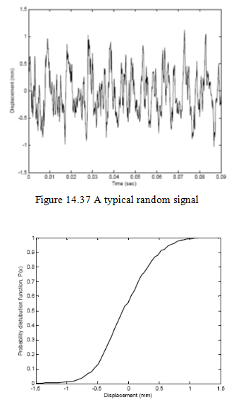
Figure 14.38 The probability distribution function

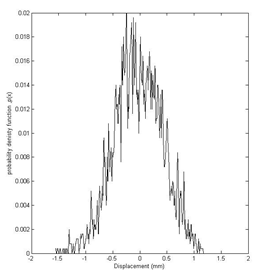
Figure 14.39 The probability density