As the probability can be added, they can also be subtracted. The probability of any randomly selected displacement having a magnitude between two limits x1 and x2 can be written as
|
(14.40) |
The probability that X lies between x and x + dx can be written as
|
(14.41) |
For dx to be infinitesimal, we have
|
(14.42) |
where p(x) is called the probability density function, which is an alternate way of describing the probability distribution of a random variable, x. Figure 14.39 shows the probability density of the random displacement signal shown in Figure 14.37. Subsequently, it will be shown that how fluctuation in p(x) can be improved. Equation (14.42) can be expressed as
|
(14.43) |
Suppose we want to know the steady and fluctuating component of our signal. The steady component is simply the mean value or expectation E[x(t)] of x(t). Noting equation (14.39), on similar analogy we can write
|
(14.44) |
where square brackets indicate the ensemble average of the quantity. It can be seen that E[x(t)] is given by the position of the centroid of the p(x) diagram, since
|
(14.45) |
During estimation of p(x) no assumption of standard p(x) (i.e., Gaussian, Raleigh, etc.) is applied. For example with the standard Gaussian p(x), it can be obtained by the use of mean and standard deviation of the signal.
14.9.2 Random Process, Ensemble, and Sample Function
The central notion involved in the concept of a random process x(t) is that not just one time history is described but the whole family or ensemble of possible time histories which might have been the outcome of the same experiment are described. Any single individual time history belonging to the ensemble is called a sample function. A random process can have several sample functions x(j)(t) (j = 1,2,...,n) defined in the same time interval (see Fig. 14.40). Each x(j)(t) is a sample function of the ensemble. Hence, a random process can be thought of as an infinite ensemble of sample functions.
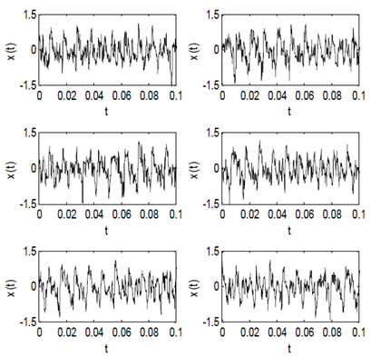
Figure 14.40 Ensemble of sample functions x(j)(t)