where n is the number of nodes in the entire shaft. Here we can see that unlike the previous example, here every element of the force vector is having a fixed force value. This is due to the helical distribution of unbalance throughout the shaft.

Figure 13.40 shows the initial unbalance responses (both the amplitude and the phase) with the spin speed of the rotor when only residual unbalances are present, and there are no trial (or correction) masses placed on balancing planes. It represents the imbalance response generated by the residual unbalance forces on the two measuring planes near bearing locations. For these responses no damping and no noise is added.

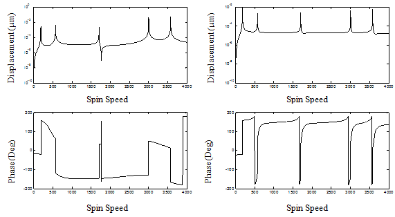
Fig. 13.40 Variation of the unbalance response amplitude and phase with the spin speed (with residual unbalances, without damping, and no noise) (left) for the left measuring plane (right) for the right measuring plane

Figure 13.41 shows plots of unbalance responses with the damping. It can be observed that due to the damping, amplitudes of unbalance responses have decreased; especially the higher modes have diminished much. Now the noise of the order of 3% and 5% is added to these responses to mimic the measurement noise in these responses, and Figs. 13.42 and 13.43 show the respective plots. However, it can be observed from these graphs with even 3% and 5% noises, they look closer to the plots with no noise case; however, the estimation of residual unbalances affects due to the presence of noise.

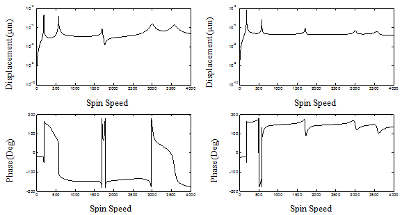
Fig. 13.41 Variation of the unbalance response amplitude and phase with the spin speed (residual unbalances, with damping and no noise) (left) for the left measuring plane (right) for the right measuring plane

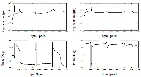
Fig. 13.42 Variation of the unbalance response amplitude and phase with the spin speed (residual unbalances, with damping and 3% noise) (left) for the left measuring plane (right) for the right measuring plane