Experimental Determination of Influence Coefficients: Influence coefficient matrix can be obtained by attaching a trial mass in balancing planes alternatively and measuring displacement at various measuring planes, from equation (13.50), we get for a particular speed

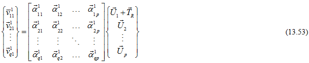
where the second subscript represents corresponding to measurements while keeping the trial mass at that plane. It is assumed that the influence coefficients do not change by adding a small trial masses during the measurement. On subtracting equation (13.53)from first q equation in equation (13.50) , we get

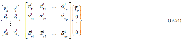
Equation (13.54) gives

Similarly, by attaching a trial mass on plane 2 we get second column of the influence coefficient matrix in equation (13.55), the above analysis should be done at a constant speed. Similarly we can find the influence coefficient matrix for other speeds.

Example 13.6 For the balancing of a flexible rotor as shown in Fig. 13.30 and corresponding data given in Table 13.1. Take discs as the two balancing planes. For the numerical simulation, two residual unbalances of 3 gm at 0º and 5 gm at 240º are considered on discs. In addition to these continuous distribution of eccentricity of the shaft is considered in a form of a spiral. The aim would be to obtain net effects of these using only simulated responses for different trial runs with additional trial unbalances. Generate unbalance responses with respect to spin speeds for speed above the second critical speed of the shaft at locations 5 cm from each of the bearings using the finite element method. Using a trial mass of 4 gm at 40º first in disc 1 and then in disc 2, generate another sets of unbalance responses for the same speed range. Obtain and plot the variation of various influence coefficients with the spin speed of the rotor. Then estimate back net residual unbalances (assumed initially discrete as well as continuous) of the rotor system at discs 1 and 2 to balance the rotor up to second flexible modes. To mimic the actual experimentation different level of random noise (1 to 5 %) may be added to the numerically simulated unbalance responses. Consider bearings as simply supported.

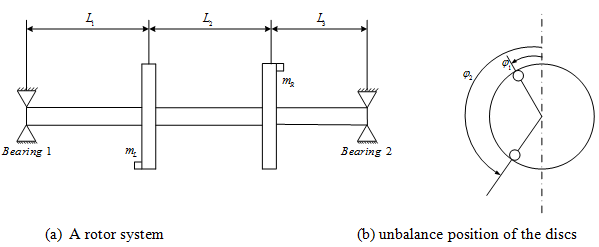
Fig. 13.31 A rotor system with two balancing planes and continuous distribution of unbalance on the shaft

Table 13.4 Data for the rotor shaft system with helical distribution of unbalance

Sl. No.	Property	Assumed value
1	Diameter of the shaft	10 mm
2	Young’s modulus of the shaft and disc materials	2.1x1011 N/m2
3	Length of the entire shaft	0.409 m
4	Distance  between left bearing and left disc	0.1375 m
5	Distance  between the two discs	0.157 m
6	Distance  between the right disc and the right bearing	0.1145 m
7	Mass of each of the balancing disc is	800 gm
8	Density of the material of the shaft	7800kg/m3
9	The trial mass kept on both discs one by one	4 gm
10	The phase angle of the trial mass of the disc	40º
11	The eccentricity of the trial mass on the disc	37 mm
12	The outer diameter of the rigid disc	60 mm
13	The inner diameter of the rigid disc	10 mm
14	The speed range in which all the calculation is done	0 - 4000 rad/s
15	The eccentricity of the unbalance in the shaft	0.2 mm