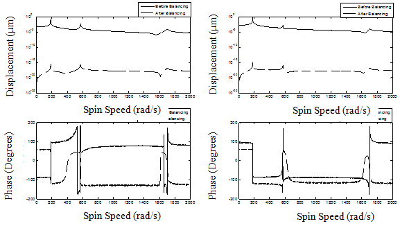
Fig. 13.39 Plot after balancing with damping and 5% noise.

Fig. 13.26 shows the superposed plots of the response plotted before balancing and that plotted after balancing. Here neither damping nor noise is considered.  The plot reveals that the rotor is balanced and the phase also changes accordingly. Figs. 13.27 to 13.29 give the plot of responses in different conditions involving damping and noise. Figure 13.28 and 13.29 show the case of balancing with three and five percent noises, respectively. So from the graphs it is evident that even with five percent noise it is possible to balance the rotor.

Example 13.7 For the rotor system of Example 13.6, let us consider a distributed unbalance (e.g., spiral eccentricity) on the shaft in addition to concentrated unbalances at disc locations. Do the dynamic balancing of the rotor up to second mode by the influence coefficient method.

Solution: As for as formulation is considered it is similar to Example 13.7 in all respect except the way the external force vector is calculated. In the case of rotor with discrete unbalance the net external force vector is given by the following relation

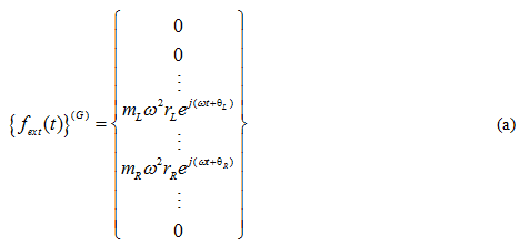
The position of the left and right unbalance forces are given by the position of the balancing plane. Since there is no unbalance in other shaft elements therefore other elements have zero forces. But now if we consider a distributed load which is in the form of a helix given by the equations

where L is the length of the shaft, z is the z-coordinate of the shaft element, and e is the eccentricity amplitude of the distributed unbalance.

Then force vector is defined by consistent load vector. (Refer Chapter 9, section 9.5.5 for detailed derivation of the consistent load matrix). In this case for a single element of the shaft consistent load vector is given by

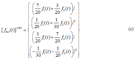
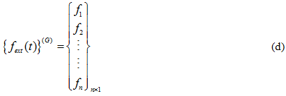
where l is the element length. After assembly, we get the consistent load vector as