Now the mass and stiffness matrix are assembled together to get the global mass and stiffness matrix. From the assembled mass and stiffness matrix we can calculate the response vector. The response vector is given by

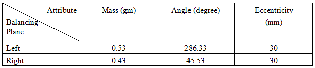
The magnitude and phase of the correction mass to be attached to the balancing planes are given in the Table 13.4.

Table 13.4: The magnitude and phase of the correction mass to be attached to the balancing

A range of speed is taken (in the present simulation, it is from 0 rad/s to 4000 rad/s) and for each speed, values of unbalance responses, both the amplitude and the phase are calculated. Now for n elements of the shaft there are (2n)unbalance responses after application of boundary conditions while considering only single plane motion. Therefore, for 10 elements of the shaft there are 20 unbalance responses. Here, it is assumed that two sensors are placed near two bearings to collect two sets of data, viz. the phase and the amplitude of unbalance responses. Two sensors are placed at node numbers  denote the node position in the shaft.

Plots of vibration amplitudes as well phase at the above two node positions are plotted in a speed range.

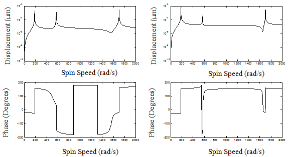
Fig. 13.32 Variation of unbalance response amplitude and phase with spin speed (with residual unbalances, without damping and zero noise) (top two) for left measuring plane (bottom two) for right measuring plane

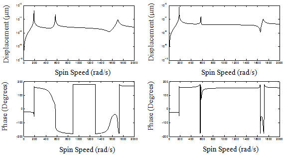
Fig. 13.33 Variation of unbalance response amplitude and phase with spin speed (residual unbalances, with damping and zero noise) (left) for left measuring plane (right) for right measuring plane