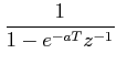
Exponential function is defined as:
We have
 |
|||
 |
Similarly Z-transforms can be computed for sinusoidal and other compound functions. One should refer the Z-transform table provided in the appendix.
2.2 Properties of Z-transform
- Multiplication by a constant:
![$ Z[ax(t)]= aX(z)$](images/img88.png) , where
, where
![$ X(z)= Z[x(t)]$](images/img89.png) .
. - Linearity: If
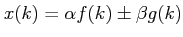 , then
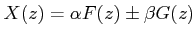 .
. - Multiplication by
 :
:
![$ Z[a^kx(k)]=X(a^{-1}z)$](images/img93.png)
- Realshifting:
![$ Z[x(t-nT)]=z^{-n}X(z)$](images/img94.png) and
and
![$ \displaystyle z[x(t+nT)]=z^{n} \left [X(z)-\sum_{k=0}^{n-1}x(kT)z^{-k} \right ]$](images/img95.png)
Complex shifting:![$ Z[e^{\pm at}x(t)]=X(ze^{\mp aT})$](images/img96.png)
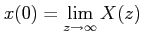
- Initial value theorem:
- Final value theorem:
![$\displaystyle \lim_{k\rightarrow\infty}x(k)= \lim_{z\rightarrow 1}[(1-z^{-1})X(z)] $](images/img98.png)