if, $s=\sigma+jw$ ,

$\displaystyle Re \; z$	= $\displaystyle e^{T\sigma}\cos wT$
$\displaystyle Im \; z$	= $\displaystyle e^{T\sigma}\sin wT$

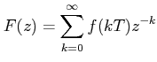
Z-transform:

$\displaystyle F^{*}\left[s=\frac{1}{T}ln \; z\right]$	= $\displaystyle F(z)$
	$\displaystyle =$ $\displaystyle \sum_{k=0}^{\infty}f(kT)z^{-k}$

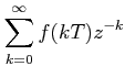F(z), is the Z-transform of f(t) at the sampling instants k

$\displaystyle F(z)=\sum_{k=0}^{\infty}f(kT)z^{-k}$

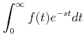
In general, we can say that if f(t) is Laplace transformable then it also has a Z-transform.

$\displaystyle L[f(t)]$	= $\displaystyle \int_{0}^{\infty}e^{-st}dt$
$\displaystyle Z[f(t)]$	= $\displaystyle \sum_{k=0}^{\infty}f(kT)z^{-k}$