2. Revisiting Z-Transforms

Z-transform is a powerful operation method to deal with discrete time systems. In considering Z-transform of a time function x(t), we consider only the sampled values of x(t), i.e., x(0), x(T), x(2T)........... where T is the sampling period.

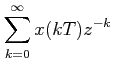$\displaystyle X(z)=Z[x(t)]$	= $\displaystyle Z[x(kT)]$
	= $\displaystyle \sum_{k=0}^{\infty}x(kT)z^{-k}$

For a sequence of numbers x(k)

$\displaystyle X(z)$	= $\displaystyle Z[x(k)]$
	= $\displaystyle \sum_{k=0}^{\infty}x(k)z^{-k}$

The above transforms are referred to as one sided z-transform. In one sided z-transform, we assume that x(t) = 0 for t < 0 or x(k) = 0 for k< 0. In two sided z-transform, we assume that - ∞ < t < ∞ or k = , ±1,±2, ±3, ................

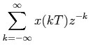$\displaystyle X(z)$	= $\displaystyle Z[x(kT)]$
	= $\displaystyle \sum_{k=-\infty}^{\infty}x(kT)z^{-k}$

or for x(k)

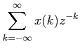$\displaystyle X(z)$	= $\displaystyle Z[x(k)]$
	= $\displaystyle \sum_{k=-\infty}^{\infty}x(k)z^{-k}$