Equations of motion for element (2) can be written as
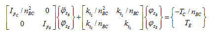 |
(b) |
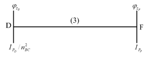
Element (3): Figure 7.28 shows element (3) with nodal variables. Here also instead of actual rotational displacement of gear D the rotational displacement of gear B is used.
For element (3), we can write the equation of motion as
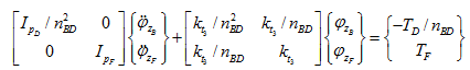 |
(c) |
In the present problem we have discretised the system into three elements. However, because at the branched point rotational displacements of three gears (i.e., B, C, D) are related, and this leads to a finite element system model of only four-DOF system. Hence, on assembling equations (a-c), we get
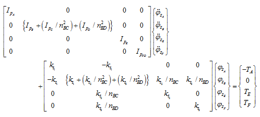 |
(d) |
It should be noted that in the assembled form, the second row in the torque column is zero, since we have the following condition at the branch point
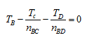 |
(e) |
From free boundary conditions at shaft ends A, E and F, we have
(f) |
Hence, on application of boundary conditions in equation (d), all the terms in the right hand side vector are zero. Hence, equation (d) forms an eigen value problem with the matrix size of 4×4. From equation (d), now to have torsional natural frequencies, we have
(g) |
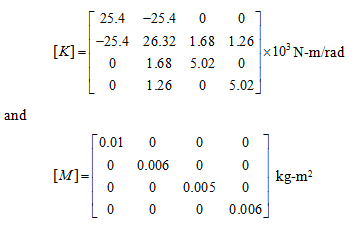
where [ K ] and [ M ] are the assembled stiffness and mass matrices. Equation (g) gives frequency equation as a polynomial and roots of the polynomial gives torsional natural frequency of the system. However, for a matrix of size 4 ´ 4 it is quite cumbersome. Alternatively, equation (g) could be written as
(h) |
In which eigen value of matrix [ D ] is related with natural frequencies (square root of the eigen value is the natural frequency) and eigen vector is related with mode shape. Hence, this method requires eigen value analysis and it is preferred for large size matrices. It should be noted that the stiffness matrix, [ K ], is a singular matrix since we have free-free boundary conditions. For the present case, we have following data
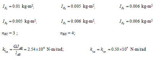
The assembled stiffness and mass matrices will have the following form