Exercise Problems

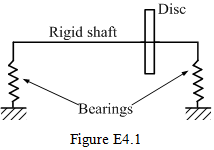
Exercise 4.1 Obtain bending critical speeds of a rotor as shown in Figure E4.1. It consists of a massless rigid shaft (1 m of span with 0.7 m from the disc to the left bearing), a rigid disc (5 kg of the mass and 0.1 kg-m2 of the diametral mass moment of inertia) and supported on two identical flexible bearings (1 kN/m of stiffness for each bearing). Consider the motion in vertical plane only. Is there is any difference in critical speeds when the disc is placed at the centre of the rotor? If NO then justify the same and if YES then obtain the same. [Hint: When the disc at the centre of the shaft-span then the uncoupled linear and angular motions would take place.]

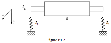
Exercise 4.2: Consider a long rigid rotor, R, supported on two identical bearings, B₁ and B₂, as shown in Figure E4.2. The direct stiffness coefficients of both bearings in the horizontal and vertical directions are equal, i.e. K. Take the direct damping, and the cross-coupled stiffness and damping coefficients of both bearings negligible. The mass of the rotor is m, the span of the rotor is l, and the diametral mass moment of inertia is I_d. Derive equations of motion, and obtain natural frequencies of whirl. Neglect the gyroscopic effect

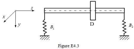
Exercise 4.3 Find critical speeds of the rotor bearing system shown in Figure E4.3. The shaft is rigid and massless. The mass of the disc is: m_d = 1 kg with negligible diamentral mass moment of inertia. Bearings B₁ and B₂ are identical bearings and have following properties: k_xx = 1.1 kN/m, k_yy = 1.8 kN/m, k_xy = 0.2 kN/m, and k_yx = 0.1 kN/m. Take: B₁D = 75 mm, and DB₂ = 50 mm.

Exercise 4.4 For exercise 4.3 take 25 g-mm of the unbalance in the disc at 380 from a shaft reference point. Plot the disc response amplitude and phase to show all critical speeds. Plot the variation of bearing forces with the spin speed of rotor.

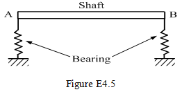
Exercise 4.5 Obtain transverse critical speeds of a rotor-bearing system as shown in Figure E4.5. Consider the shaft as a rigid and the whole mass of the shaft is assumed to be concentrated at its mid-span. The shaft is of 1 m of span and the diameter is 0.05 m with the mass density of 7800 kg/m3. The shaft is supported at ends by flexible bearings. Consider the motion in both the vertical and horizontal planes. Take the following bearing properties: For bearing A: k_xx = 200 MN/m, k_yy = 150 MN/m, k_xy = 15 MN/m, k_yx = 10 MN/m, c_xx = 200 kN-s/m, c_yy = 150 kN-s/m, c_xy = 14 kN-s/m, c_yx = 21 kN-s/m, and for bearing B: k_xx = 240 MN/m, k_yy = 170 MN/m, k_xy = 12 MN/m, k_yx = 16 MN/m, c_xx = 210 kN-s/m, c_yy = 160 kN-s/m, c_yx = 13 kN-s/m, c_yy = 18 kN-s/m. Use a numerical simulation to get the unbalance response to cross check the critical speeds for an assumed unbalance.

Exercise 4.6 For exercise 4.5 consider the shaft as flexible and attach a rigid disc of 10 kg on the shaft at a distance of 0.6 m from the end A. Obtain the transverse critical speeds of the system by attaching an unbalance on the disc. Take 40 g-mm of the unbalance in the disc at 130° from a shaft reference point.

Exercise 4.7 For exercise 4.5 obtain critical speeds of the rotor-bearing-foundation system when the foundation has the following dynamic characteristics: Take the mass of each bearing as 2 kg. Plot the unbalance response amplitude and phase of the shaft end and the bearing at A with respect to the spin speed of shaft to show all critical speeds of the system. Take 25 g-mm of the unbalance in the disc at 380 from a shaft reference point. Plot also the variation of the bearing and foundation forces at A with the spin speed.

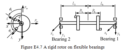
Exercise 4.8 Consider a simple rigid rotor-bearing system as shown in Figure E4.7. The rotor is supported on two different flexible bearings. In Figure E4.7, L₁ and L₂ are distances of bearings 1 and 2 from the center of gravity of the rotor with L = L₁ + L₂, R₁ and R₂ are distances of balancing planes (i.e., rigid discs) from the center of gravity of the rotor, and u is the unbalance. Obtain bearing dynamic parameters based on the short bearing approximations.

Let m be the mass of the rotor, I_t is the transverse mass moment of inertia of the rotor about an axis passing through the center of gravity, I_p is the polar mass moment of inertia of the rotor, k and c are respectively the stiffness and damping parameters, f_x(t) and f_y(t) are respectively the impulse in the horizontal and vertical directions, u is the unbalance, Φ is the phase, x and y are linear displacements in the horizontal and vertical directions respectively, t is the time, and subscripts 1 and 2 represent the right and left sides from the mid-span of the rotor, respectively. Obtain equations of motion of the rotor-bearing system in terms of linear displacements (four in numbers, i.e., x₁, y₁, x₂, y₂) at two bearings. The motivation behind obtaining the equations of motion in terms of bearing response is that in practical situation often these responses can only be accessible to the practicing engineers.

[Hint: The linearised equation of motion of the rotor-bearing system is given as

where ω is the shaft rotational speed, {ƒ}_Runb is the residual unbalance force vector, {q} is the displacement response vector, and matrices [M], [C] and [K] are the mass, damping, and stiffness matrices and are given as

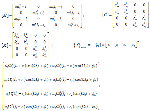
with