We have seen that transform domain analysis of a digital control system yields a transfer function of the following form.

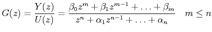$\displaystyle G(z)=\frac{Y(z)}{U(z)}=\frac{\beta_0z^m+\beta_1z^{m-1}+\ldots+\beta_m}{z^n+\alpha_1z^{n-1}+\ldots+\alpha_n} \quad m\le n$

(3)

Various canonical state variable models can be derived from the above transfer function model.

Consider the transfer function as given in Eqn. (3). Without loss of generality, we assume . Let

$\displaystyle \frac{\bar X(z)}{U(z)}=\frac{1}{z^n+\alpha_1z^{n-1}+\ldots+\alpha_n}$

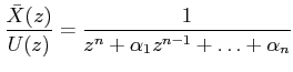
In time domain, the above equation may be written as

$\displaystyle \bar x(k+n)+\alpha_1 \bar x(k+n-1)+\ldots+\alpha_n \bar x(k)=u(k)$

Now, the output may be written in terms of $\bar X(z)$ as

$\displaystyle Y(z)=\left(\beta_0z^n+\beta_1z^{n-1}+\ldots+\beta_n\right)\bar X(z)$

or in time domain as

$\displaystyle y(k)=\beta_0 \bar x(k+n)+\beta_1 \bar x(k+n-1)+\ldots+\beta_n \bar x(k)$

The block diagram representation of above equations is shown in Figure 1. State variables are selected as shown in Figure 1.