In this lecture we will discuss about the relation between transfer function and state space model for a discrete time system and various standard or canonical state variable models.

1 State Space Model to Transfer Function

Consider a discrete state variable model

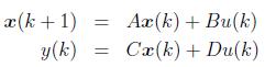(1)

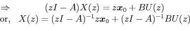
Taking the Z-transform on both sides of Eqn. (1), we get

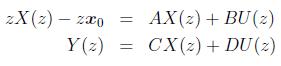where $\boldsymbol{x}_0$ is the initial state of the system.

$\begin{displaymath} \begin{array}{cc} \Rightarrow & (zI-A) X(z) = z \boldsymbol... ...) = (zI-A)^{-1} z \boldsymbol{x}_0+(zI-A)^{-1}BU(z) \end{array}\end{displaymath}$

To find out the transfer function, we assume that the initial conditions are zero, i.e.,

, thus

$\displaystyle Y(z)=\Big(C(zI-A)^{-1}B+D\Big)U(z)$

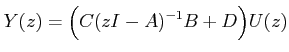
Therefore, the transfer function becomes

$\displaystyle G(z)=\frac{Y(z)}{U(z)}=C(zI-A)^{-1}B+D$

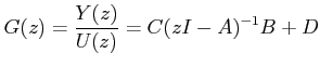(2)

which has the same form as that of a continuous time system.