Module 2 : Modeling Discrete Time Systems by Pulse Transfer Function

Lecture 3 : Pluse Transfer Function

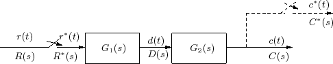
Figure 3 shows the block diagram for the second case.

Figure 3: Discrete data system with cascaded elements, not separated by a sampler
\begin{figure}\centering
\input{m2fig3.pstex_t}\end{figure}

The continuous output $ C(s)$ can be written as

$\displaystyle C(s) = G_1(s) G_2(s) R^*(s) $

The output of the fictitious sampler is

$\displaystyle C(z) = Z\left [G_1(s)G_2(s) \right ] R(z) $

z-transform of the product $ G_1(s)G_2(s)$ is denoted as

$\displaystyle Z\left [G_1(s)G_2(s) \right ] = G_1G_2(z) = G_2G_1(z) $

One should note that in general $ G_1G_2(z)\ne G_1(z) G_2(z) $, except for some special cases. The overall output is thus,

$\displaystyle C(z) = G_1G_2(z)R(z) $