1. Pluse Transfer Function

Transfer function of an LTI (Linear Time Invariant) continuous time system is defined as

$\displaystyle G(s)=\frac{C(s)}{R(s)}$

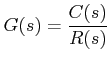
where R(s) and C(s) are Laplace transforms of input r(t) and output c(t). We assume that initial condition are zero.

Pulse transfer function relates Z-transform of the output at the sampling instants to the Z- transform of the sampled input.

When the same system is subject to a sampled data or digital signal r*(t), the corresponding block diagram is given in Figure 1 .

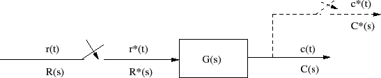
**Figure 1:** Block diagram of a system subject to a sampled input
$\begin{figure}\centering \input{m2fig1.pstex_t}\end{figure}$

The output of the system is C(s) = G(s)R*(s). The transfer function of the above system is difficult to manipulates because it contains a mixture of analog and digital components. Thus, for ease of manipulation, it is desirable to express the system characteristics by a transfer function that relates r*(t) to c*(t), a fictitious sampler output, as shown in Figure 1.