To justify D at output of gate-1, if we use backward implication we get a =1 and b =1. In other words, backward implication in gate-1 (J-frontier) generates a =1 and b =1. This step is illustrated in Figure 7(c). Now, J-frontier has no gates.

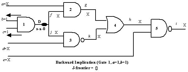Figure 7(c): Backward implication at gate-1

If we observe Figure 7(b), we see that there are 2 gates in D-frontier, namely 2 and 3. So we can choose one for fault propagation. Let us first try gate 2. So net f =D and j =X. This is illustrated in Figure 7(d).  Now, gate 3 is removed from D-frontier and only gate 2 remains.
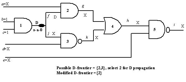                                         Figure 7(d): Selection of gate-2 as D-frontier

In the next step, we propagate D though gate-2 (only choice in the D-frontier). This makes net g =D by forward implication and a =1 by backward implication. The step is illustrated in Figure 7(e). After propagation of D though gate-2, the new D-frontier comprises gate-4.

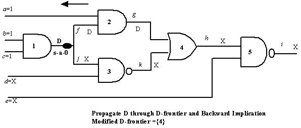
 Figure 7(e): Propagation of D and implications

In the next step, we propagate D through gate-4 (only choice in the D-frontier). This makes net h = D by forward implication. So D-frontier comprises gate-5. Now by backward implication net k = 0. This creates a new J-frontier comprising gate-3; output of gate-3 is 0 and both of its inputs are X. The step is illustrated in Figure 7(f).
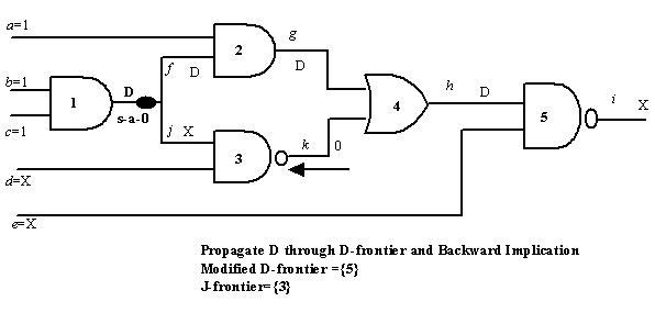                               Figure 7(f): Propagation of D, implications and J-frontier