Figure 3 explains the forward implication procedure. 

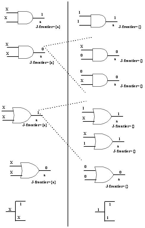
Figure 3. Backward implication and J-frontier

In Figure 3, gates at left side represent the case before backward implication and the ones at the right side illustrate the situation after implication The first gate in the sequence (from top) has inputs as X and output as 1; so J-frontier is a. Now by backward implication (i.e., singular cover) both inputs are to be 1. The corresponding gate in right side shows that inputs are decided by backward implication and so gate (a) is removed from J-frontier. In Figure 3, the second gate has output of 0 and so by singular cover we have two options for assigning values to the inputs; the two options are shown in the right side. It may be noted that we could have also kept another option where both the inputs are kept 1. However, this is avoided because if both inputs are fixed then flexibility gets reduced and chances of inconsistency increases. This is explained by an example given in Figure 4. In the figure it may be noted that in Step-2 we have three options (at the input) to obtain D at the output of the AND gate--00,01 and 10.  If we choose 10 then we will have inconsistency in Step-4, because to propagate D through the OR gate the input not carrying D is to be 0. To avoid such   inconsistencies we maintain as many X as possible to have flexibility for successful forward and backward implications. 

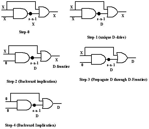
Figure 4. Propagating D using backward and forward implication