| |
| | |
|
The delay model incorporated into the HCM 2000 includes the uniform delay
model, a version of Akcelik's overflow delay model, and a term covering delay
from an existing or residual queue at the beginning of the analysis period.
The delay is given as,
 additional explanation for PF
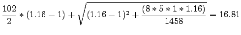
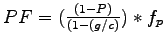
Where, d = control delay, s/veh, d1 = uniform delay component, s/veh, PF = progression adjustment factor, d2 = overflow delay component, s/veh, d3 = delay due to pre-existing queue, s/veh, T = analysis period, h, X = v/c ratio, C = cycle length, s, k = incremental delay factor for actuated controller settings; 0.50 for all pre-timed controllers, l = upstream filtering/metering adjustment factor; 1.0 for all individual intersection analyses, c = capacity, veh/h, P = proportion of vehicles arriving during the green interval and additional explanation for PF
Where, d = control delay, s/veh, d1 = uniform delay component, s/veh, PF = progression adjustment factor, d2 = overflow delay component, s/veh, d3 = delay due to pre-existing queue, s/veh, T = analysis period, h, X = v/c ratio, C = cycle length, s, k = incremental delay factor for actuated controller settings; 0.50 for all pre-timed controllers, l = upstream filtering/metering adjustment factor; 1.0 for all individual intersection analyses, c = capacity, veh/h, P = proportion of vehicles arriving during the green interval and  = supplemental adjustment factor for platoon arriving during the green
Consider the following situation: An intersection approach has an approach flow rate of 1,400 vph, a saturation flow rate of 2,650 vphg, a cycle length of 102 s, and effective green ratio for the approach 0.55.
Assume Progression Adjustment Factor 1.25 and delay due to pre-existing queue, 12 sec/veh.
What control delay sec per vehicle is expected under these conditions?
Saturation flow rate =2650 vphg , g/C=0.55, Approach flow rate v=1700 vph, Cycle length C=102 sec, delay due to pre-existing queue =12 sec/veh and Progression Adjustment Factor PF=1.25.
The capacity is given as: = supplemental adjustment factor for platoon arriving during the green
Consider the following situation: An intersection approach has an approach flow rate of 1,400 vph, a saturation flow rate of 2,650 vphg, a cycle length of 102 s, and effective green ratio for the approach 0.55.
Assume Progression Adjustment Factor 1.25 and delay due to pre-existing queue, 12 sec/veh.
What control delay sec per vehicle is expected under these conditions?
Saturation flow rate =2650 vphg , g/C=0.55, Approach flow rate v=1700 vph, Cycle length C=102 sec, delay due to pre-existing queue =12 sec/veh and Progression Adjustment Factor PF=1.25.
The capacity is given as:
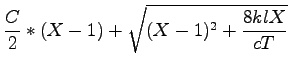
Degree of saturation X= v/c= 1700/1458 =1.16.
So the uniform delay is given as:
Uniform delay =22.95 and the over flow delay is given as:
Overflow delay, d2=16.81.
Hence, the total delay is"
Therefore, control delay per vehicle is 53.5 sec.
|
|
| | |
|
|
|
![$\displaystyle \frac{c}{2}\frac{(1-\frac{g}{c})^2}{1-[min(1,X)(\frac{g}{c})]}$](img5.png)
![$\displaystyle 900T[(X-1)+\sqrt{(X-1)^2+\frac{8klX}{cT}}]$](img7.png)

![$\displaystyle \frac{C}{2}\frac{(1-\frac{g}{C})^2}{[1-min(X,1)(\frac{g}{c})]}$](img14.png)
![$\displaystyle \frac{102}{2}\frac{(1-1.16)^2}{[1-min(1.16,1)(.55)]}= 22.95$](img15.png)