Module 7 : Traffic Signal Design

Lecture 35 : Signalized Intersection Delay Models

1

2

3

4

5

6

7

8

9

	Components of delay In analytic models for predicting delay, there are three distinct components of delay, namely, uniform delay, random delay, and overflow delay. Before, explaining these, first a delay representation diagram is useful for illustrating these components. Delay diagram All analytic models of delay begin with a plot of cumulative vehicles arriving and departing vs. time at a given signal location. Fig. 1 shows a plot of total vehicle vs time. Two curves are shown: a plot of arriving vehicles and a plot of departing vehicles. The time axis is divided into periods of effective green and effective red. Vehicles are assumed to arrive at a uniform rate of flow ($v$ vehicles per unit time). This is shown by the constant slope of the arrival curve. Uniform arrivals assume that the inter-vehicle arrival time between vehicles is a constant. Assuming no preexisting queue, arriving vehicles depart instantaneously when the signal is green (ie., the departure curve is same as the arrival curve). When the red phase begins, vehicles begin to queue, as none are being discharged. Thus, the departure curve is parallel to the x-axis during the red interval. When the next effective green begins, vehicles queued during the red interval depart from the intersection, at a rate called saturation flow rate ($s$ vehicle per unit time). For stable operations, depicted here, the departure curve catches up with the arrival curve before the next red interval begins (i.e., there is no residual queue left at the end of the effective green). Figure 1: Illustration of delay, waiting time, and queue length 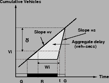In this simple model: The total time that any vehicle ($v_i$) spends waiting in the queue ($W_i$) is given by the horizontal time-scale difference between the time of arrival and the time of departure. 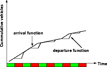The total number of vehicles queued at any time ($q_t$) is the vertical vehicle-scale difference between the number of vehicles that have arrived and the number of vehicles that have departed The aggregate delay for all vehicles passing through the signal is the area between the arrival and departure curves (vehicles times the time duration) Uniform Delay Uniform delay is the delay based on an assumption of uniform arrivals and stable flow with no individual cycle failures. Fig. 2, shows stable flow throughout the period depicted. No signal cycle fails here, i.e., no vehicles are forced to wait for more than one green phase to be discharged. During every green phase, the departure function catches up with the arrival function. Total aggregate delay during this period is the total of all the triangular areas between the arrival and departure curves. This type of delay is known as Uniform delay. 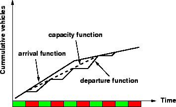Figure 2: Illustration of uniform delay Random Delay Random delay is the additional delay, above and beyond uniform delay, because flow is randomly distributed rather than uniform at isolated intersections. In Fig 3some of the signal phases fail. At the end of the second and third green intervals, some vehicles are not served (i.e., they must wait for a second green interval to depart the intersection). By the time the entire period ends, however, the departure function has caught up with the arrival function and there is no residual queue left unserved. This case represents a situation in which the overall period of analysis is stable (ie.,total demand does not exceed total capacity). Individual cycle failures within the period, however, have occurred. For these periods, there is a second component of delay in addition to uniform delay. It consists of the area between the arrival function and the dashed line, which represents the capacity of the intersection to discharge vehicles, and has the slope c. This type of delay is referred to as Random delay. 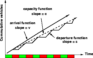Figure 3: Illustration of random delay Overflow Delay Overflow delay is the additional delay that occurs when the capacity of an individual phase or series of phases is less than the demand or arrival flow rate. Fig. 4 shows the worst possible case, every green interval fails for a significant period of time, and the residual, or unserved, queue of vehicles continues to grow throughout the analysis period. In this case, the overflow delay component grows over time, quickly dwarfing the uniform delay component. The latter case illustrates an important practical operational characteristic. When demand exceeds capacity ($v/c >1.0$), the delay depends upon the length of time that the condition exists. In Figure 3, the condition exists for only two phases. Thus, the queue and the resulting overflow delay is limited. In Fig. 4, the condition exists for a long time, and the delay continues to grow throughout the over-saturated period. This type of delay is referred to as Overflow delay Figure 4: Illustration of overflow delay