| |
| | |
|
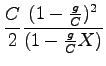
The uniform delay model assumes that arrivals are uniform and that no signal
phases fail (i.e., that arrival flow is less than capacity during every signal
cycle of the analysis period).
At isolated intersections, vehicle arrivals are more likely to be random.
A number of stochastic models have been developed for this case, including those
by Newell, Miller and Webster.
These models generally assume that arrivals are Poisson distributed, with an
underlying average rate of v vehicles per unit time.
The models account for random arrivals and the fact that some individual cycles
within a demand period with  could fail due to this randomness.
This additional delay is often referred to as Random delay.
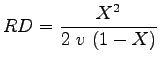
The most frequently used model for random delay is Webster's formulation: could fail due to this randomness.
This additional delay is often referred to as Random delay.
The most frequently used model for random delay is Webster's formulation:
 |
(1) |
where,
RD is the average random delay per vehicle, s/veh, and
X is the degree of saturation (v/c ratio).
Webster found that the above delay formula overestimate delay and hence he
proposed that total delay is the sum of uniform delay and random delay multiplied by a constant for agreement with field observed values.
Accordingly, the total delay is given as:
 |
(2) |
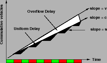
Model is explained based on the assumption that arrival function is uniform.
In this model a new term called over saturation is used to describe the extended
time periods during which arrival vehicles exceeds the capacity of the
intersection approach to the discharged vehicles.
In such cases queue grows and there will be overflow delay in addition to the
uniform delay.
Fig. 1 illustrates a time period for which  . .
Figure 1:
Illustration of overflow delay model
 |
During the period of over-saturation delay consists of both uniform delay (in the
triangles between the capacity and departure curves) and overflow delay (in the
triangle between arrival and capacity curves).
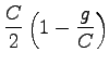
As the maximum value of X is 1.0 for uniform delay, it can be simplified as,
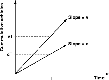
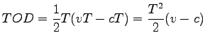
From Fig. 2 total overflow delay can be estimated as,
Figure 2:
Derivation of the overflow delay model
 |
 |
(4) |
where,
TOD is the total or aggregate overflow delay (in veh-secs), and
T is the analysis period in seconds.
Average delay is obtained by dividing the aggregate delay by the number of
vehicles discharged with in the time T which is cT.
 |
(5) |
The delay includes only the delay accrued by vehicles through time T, and
excludes additional delay that vehicles still stuck in the queue will
experience after time T.
The above said delay equation is time dependent i.e., the longer the period of
over-saturation exists, the larger delay becomes.
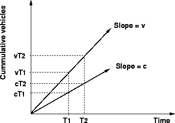
A model for average overflow delay during a time period T1 through T2 may be
developed, as illustrated in Fig. 3 Note that the delay
area formed is a trapezoid, not a triangle.
The resulting model for average delay per vehicle during the time period T1
through T2 is:
 |
(6) |
Figure 3:
Overflow delay between time T1 & T2
 |
Formulation predicts the average delay per vehicle that occurs during the
specified interval,  through through  .
Thus, delays to vehicles arriving before time but discharging after
are included only to the extent of their delay within the specified times, not
any delay they may have experienced in queue before .
Similarly, vehicles discharging after are not included in the formulation.
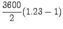
Consider the following situation: An intersection approach has an approach flow
rate of 1,900 vph, a saturation flow rate of 2,800 vphg, a cycle length of 90s,
and effective green ratio for the approach 0.55.
What average delay per vehicle is expected under these conditions?
To begin, the capacity and v/c ratio for the intersection approach must be
computed.
This will determine what model(s) are most appropriate for application in this
case:
Given,
s=2800 vphg, g/C=0.55, and v =1900 vph. .
Thus, delays to vehicles arriving before time but discharging after
are included only to the extent of their delay within the specified times, not
any delay they may have experienced in queue before .
Similarly, vehicles discharging after are not included in the formulation.
Consider the following situation: An intersection approach has an approach flow
rate of 1,900 vph, a saturation flow rate of 2,800 vphg, a cycle length of 90s,
and effective green ratio for the approach 0.55.
What average delay per vehicle is expected under these conditions?
To begin, the capacity and v/c ratio for the intersection approach must be
computed.
This will determine what model(s) are most appropriate for application in this
case:
Given,
s=2800 vphg, g/C=0.55, and v =1900 vph.
Since v/c is greater than 1.15 for which the overflow delay model is good so it
can be used to find the delay.
This is a very large value but represents an average over one full hour period.
|
|
| | |
|
|
|