| |
| | |
|
The most commonly used model for intersection delay is to fit models that works well under all v/c ratios.
Few of them will be discussed here.
To address the above said problem Akcelik proposed a delay model and is used in the Australian Road Research Board's signalized intersection.
In his delay model, overflow component is given by,
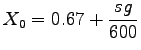
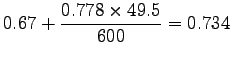
where  , and if , and if  then overflow delay is zero, and then overflow delay is zero, and
 |
(1) |
where,
T is the analysis period, h,
X is the v/c ratio,
c is the capacity, veh/hour,
s is the saturation flow rate, veh/sg (vehicles per second of green) and
g is the effective green time, sec
Consider the following situation: An intersection approach has an approach flow
rate of 1,600 vph, a saturation flow rate of 2,800 vphg, a cycle length of 90s,
and a g/C ratio of 0.55.
What average delay per vehicle is expected under these conditions?
To begin, the capacity and v/c ratio for the intersection approach must be
computed.
This will determine what model(s) are most appropriate for application in this
case:
Given, s =2800 vphg; g/C=0.55; v =1600 vph
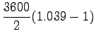
In this case, the v/c ratio now changes to 1600/1540 = 1.039.
This is in the difficult range of 0.85-1.15 for which neither the simple random
flow model nor the simple overflow delay model are accurate.
The Akcelik model of Equation will be used.
Total delay, however, includes both uniform delay and overflow delay.
The uniform delay component when  is given by equation is given by equation ![[*]](file:/usr/local/share/lib/latex2html/icons/crossref.png)
Use of Akcelik's overflow delay model requires that the analysis period be
selected or arbitrarily set.
If a one-hour
The total expected delay in this situation is the sum of the uniform and
overflow delay terms and is computed as:
d=20.3+39.1=59.4 s/veh.
As in the same problem, what will happen if we use Webster's overflow delay model.
Uniform delay will be the same, but we have to find the overflow delay.
As per Akcelik model, overflow delay obtained is 39.1 sec/veh which is very much lesser compared to overflow delay obtained by Webster's overflow delay model.
This is because of the inconsistency of overflow delay model in the range 0.85-1.15.
|
|
| | |
|
|
|
![$\displaystyle OD=\frac{cT}{4}\left[(X-1)+\sqrt{(X-1)^2+\frac{12(X-X_0)}{cT}}\right]$](img1.png)

![$\displaystyle \frac{cT}{4}\left[(X-1)+\sqrt{(X-1)^2+\frac{12(X-X_0)}{cT}}\right]$](img17.png)
![$\displaystyle \frac{1540}{4}\left[(1.039-1)+\sqrt{(1.039-1)^2+\frac{12(1.039-0.734)}{1540}}\right]$](img24.png)