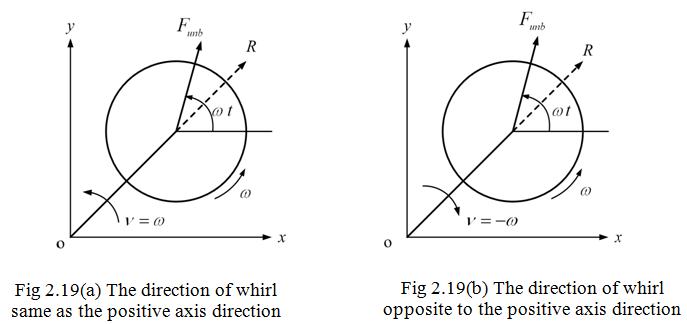
The relationship (2.57) is true for the present axis system along with directions of the whirling (R) and the unbalance force vectors chosen as shown in Figure 2.19(a). For this case  lag behind  by 90°. Let us derive this relationship: If , then

For the direction of whirl (R) opposite to the axis system as shown in Figure 2.19(b), the following relationship holds

so that,

(2.59)

in which case  lead  by 90°. It should be noted in equation (2.58) that the right hand side force vector elements have significance of real parts only, which is quite clear from the expanded form of the force vector in equation (2.56). Equation (2.58) can be written in more a compact form as

(2.60)

with

where [M] is the mass matrix, [C] is the damping matrix, [K] is the stiffness matrix, {x(t)} is the response vector, and is the unbalance force amplitude vector. The solution can be chosen as

(2.61)

where elements of the vector {X} are, in general, complex.

Equation (2.61) can be differentiated to give

(2.62)

On substituting equations (2.61) and (2.62) into equation (2.60), we get

(2.63)

with

(2.64)

where [Z] is the dynamic stiffness matrix. The response can be obtained as

(2.65)

The above method is quite general in nature and it can be applied to multi-DOF systems also once equations of motion in the standard form are available. For obtaining natural frequencies of the system directly, we need to put  to get frequency equation in the form of a polynomial. The following example illustrates the method discussed in the present section for a Jeffcott rotor.