Module 2 : Modeling Discrete Time Systems by Pulse Transfer Function

Lecture 5 : Sampled Signal Flow Graph

In Z-domain,

$\displaystyle \frac {E(z)}{R(z)}$
  $\displaystyle =$ $\displaystyle \frac{1+G_{2}H(z)}{1+G_{1}G_{2}(z)+G_{2}H(z)}$  
$\displaystyle \frac {C(z)}{R(z)}$
  $\displaystyle =$ $\displaystyle \frac{G_{1}G_{2}(z)}{1+G_{1}G_{2}(z)+G_{2}H(z)}$  

The sampled signal flow graph is not the only signal flow graph method available for discrete-data systems. The direct signal flow graph is an alternate method which allows the evaluation of the input-output transfer function of discrete data systems by inspection. This method depends on an entirely different set of terminologies and definitions than those of Mason's signal flow graph and will be omitted in this course.

Practice Problem

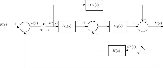
  1. Draw the composite signal flow graph of the system represented by the block diagram shown in Figure 5.
Figure 5: Block diagram for Exercise 1
\begin{figure}\centering
\input{fig_q2.pstex_t}\end{figure}

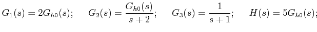
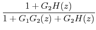
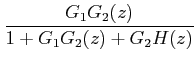
Find out the closed loop discrete transfer function $ \dfrac{C(z)}{R(z)}$ if

$\displaystyle G_1(s)= 2 G_{h0} (s); \;\;\;\;\; G_2(s)= \frac{G_{h0}(s)}{s+2};
\;\;\;\;\; G_3(s) = \frac{1}{s+1}; \;\;\;\;\; H(s) = 5 G_{h0} (s); $

where $ G_{h0}(s)$ represents zero order hold.