The input output relations:
| (3) | |||
| (4) | |||
| (5) |
The sampled SFG is shown in Figure 3(b).
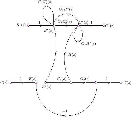
To find out the composite SFG, we take pulse transform on equations (5) and (3):
The composite SFG is shown in Figure 4.
 |
Module 2 : Modeling Discrete Time Systems by Pulse Transfer Function
Lecture 5 : Sampled Signal Flow Graph
The input output relations:
| (3) | |||
| (4) | |||
| (5) |
The sampled SFG is shown in Figure 3(b).
To find out the composite SFG, we take pulse transform on equations (5) and (3):
The composite SFG is shown in Figure 4.
|