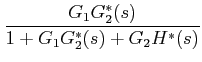
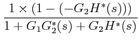
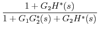
$\dfrac {C^{*}(s)}{R^{*}(s)}$ , $\dfrac {E^{*}(s)}{R^{*}(s)}$ , $\dfrac{C(s)}{R^{*}(s)}$ can be computed from Mason's gain formula, as:

$\displaystyle \frac {C^{*}(s)}{R^{*}(s)}$

$\displaystyle =$ $\displaystyle \frac {G_{1}G_{2}^{*}(s)}{1+G_{1}G_{2}^{*}(s)+G_{2}H^{*}(s)}$

$\displaystyle \frac {E^{}(s)}{R^{}(s)}$		$\displaystyle =$ $\displaystyle \frac {1 \times (1-(-G_{2}H^{}(s)))}{1+G_{1}G_{2}^{}(s)+G_{2}H^{*}(s)}$

		$\displaystyle =$ $\displaystyle \frac {1+G_{2}H^{}(s)}{1+G_{1}G_{2}^{}(s)+G_{2}H^{*}(s)}$

To derive $\displaystyle \frac {C(s)}{R^{*}(s)}$ : Number of forward paths = 2 and the corresponding gains are

	$\displaystyle \Rightarrow$	$\displaystyle 1\times 1\times G_{1}(s)\times G_{2}(s)= G_{1}(s)G_{2}(s)$
	$\displaystyle \Rightarrow$	$\displaystyle 1\times G_{1}G_{2}^{}(s)\times(-H(s))\times G_{2}(s)= -G_{2}(s)H(s)G_{1}G_{2}^{}(s)$

$\Delta_{1}=1+G_{2}H^{*}(s)$ and $\Delta_{2}=1$ .

$% latex2html id marker 642 $\displaystyle \therefore \frac {C(s)}{R^{*}(s)}=\fr... ..._{2}H^{*}(s)]-G_{2}(s)H(s)G_{1}G_{2}^{*}(s)}{1+G_{1}G_{2}^{*}(s)+G_{2}H^{*}(s)}$$