Module 2 : Modeling Discrete Time Systems by Pulse Transfer Function

Lecture 5 : Sampled Signal Flow Graph

Taking pulse transform on both sides of equations (1) and (2), we get:

$\displaystyle E^*(s)$
$\displaystyle =$ $\displaystyle R^*(s)-GH^*(s)E^{*}(s)$  
$\displaystyle C^*(s)$
$\displaystyle =$ $\displaystyle G^*(s)E^{*}(s)$  

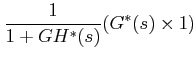
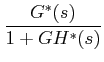
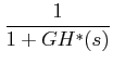
The above equations contain only discrete data variables for which the equivalent SFG will take a form as shown in Figure1(c). If we apply Mason's gain formula, we will get the following transfer functions.

$\displaystyle \frac {C^{*}(s)}{R^{*}(s)}$
$\displaystyle =$ $\displaystyle \frac {1}{1+GH^{*}(s)}(G^{*}(s)\times 1)$  
  $\displaystyle =$ $\displaystyle \frac {G^{*}(s)}{1+GH^{*}(s)}$  
$\displaystyle \frac {E^{*}(s)}{R^{*}(s)}$
$\displaystyle =$ $\displaystyle \frac{1}{1+GH^{*}(s)}$  

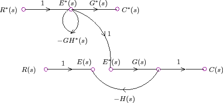
The composite signal flow graph is formed by combining the equivalent and the original sampled signal flow graphs as shown in Figure 2.

Figure 2: Composite signal flow graph for Example 1
\begin{figure}\centering
\input{m2l5f2.pstex_t}\end{figure}