1. Sampled Signal Flow Graph
It is known fact that the transfer functions of linear continuous time data systems can be determined from signal flow graphs using Mason's gain formula.
Since most discrete data control systems contain both analog and digital signals, Mason's gain formula cannot be applied to the original signal flow graph or block diagram of the system.
The first step in applying signal flow graph to discrete data systems is to express the system's equation in terms of discrete data variables only.
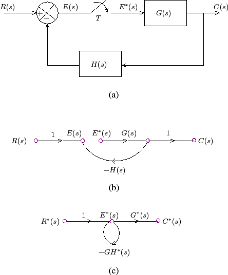
Example 1: Let us consider the block diagram of a sampled data system as shown in Figure 1(a). We can write:
| (1) | |||
| (2) |
The sampled data signal flow graph (SFG) is shown in Figure 1(b).
 |