The interconnects are illustrated in Figure 4 and can be interpreted in a similar manner as discussed for the last two cases. It may be noted that in this case we require four multiplexers in the circuit. Two multiplexers at inputs of register1 and register3 are added for the same reason as discussed in the last two cases. Now we see why two more multiplexers at inputs of both the adders are required. It may be observed from Figure 4 that data transfer “ a to operand of adder1” is binded to interconnect “register1 (source)--left input of adder1 (destination)” and “ temp2 to operand of adder1” is binded to interconnect “register3 (source)--left input of adder1 (destination)”. As there are two different interconnects for the left input of adder1, we require a multiplexer. Similarly, we require another multiplexer at input of adder2.

So, it can be concluded that depending on binding, the area taken by interconnects (including multiplexers) varies.

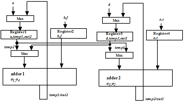
Figure 4. Case 4 of Binding for the schedule shown in Figure 1

It may also be noted that there are many allocations which are not feasible, e.g., operations 0₁,0₃ are binded to adder1, variables a,b are binded to register1 etc. This is because in a control step (step1), both the operations 0₁,0₃ need to be computed and they cannot share the same resource. Similarly, variables a,b cannot be binded to register1, because both a,b are required in control step1. As we have two addition operations in step1 (also in step2), we require two adders. Similarly, as we have four variables in step1 (also in step2), we require four registers.

So, binding process comprises two parts (for functional unit binding and variable binding), namely, (i) determination of minimal number of resources and (ii) a feasible binding. If there is more than one possible binding combinations, then the one that results in minimal area in terms of interconnects (including multiplexers) is taken as final. Now we will discuss algorithms to automate the above-mentioned two parts required for binding. It may be noted that algorithms for functional unit binding and variable binding would be very similar; so the discussion in this lecture will be on register binding. In case of functional unit binding we consider each type of operations, taking one type at a time and determine (i) minimal number of resources required for performing the operation type under question and (ii) a feasible binding of the operations with the resources. Register binding is similar to operation binding, where variables (which are binded to registers) can be considered as one type of operation. If more than one feasible binding of operations with resources (or variables with registers) is possible then the one with minimal interconnect area is considered. There exist algorithms that can determine the area of interconnects, given a legal binding, which can help in selection of the best binding [1]; we will not discuss these works in this lecture.