| |
| | |
|
An observation from 2434 samples is given table below.
Mean headway observed was 3.5 seconds and the standard deviation observed was
2.6 seconds.
Fit a normal distribution, if we assume minimum expected headway is 0.5.
Table 1:
Observed headway distribution
 |
 |
 |
| 0.0 |
1.0 |
0.012 |
| 1.0 |
2.0 |
0.178 |
| 2.0 |
3.0 |
0.316 |
| 3.0 |
4.0 |
0.218 |
| 4.0 |
5.0 |
0.108 |
| 5.0 |
6.0 |
0.055 |
| 6.0 |
7.0 |
0.033 |
| 7.0 |
8.0 |
0.022 |
| 8.0 |
9.0 |
0.013 |
| 9.0 |
 |
0.045 |
| Total |
|
1.00 |
The given headway range and the observed probability is given in column (2),
(3) and (4).
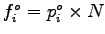
The observed frequency for the first interval (0 to 1) can be computed as the
product of observed frequency  and the number of observation (N) i.e. and the number of observation (N) i.e.
 as shown in column (5).
Compute the standard deviation to be used in calculation, given that as shown in column (5).
Compute the standard deviation to be used in calculation, given that  , ,
 , and , and
 as: as:
Second, compute the probability that headway less than zero.
The value 0.01 is obtained for standard normal distribution table is shown in
column (6).
Similarly, compute the probability that headway less than 1.0 as:
The value 0.048 is obtained from the standard normal distribution table is
shown in column (6).
Hence, the probability that headway between 0 and 1 is obtained using
equation ![[*]](file:/usr/local/share/lib/latex2html/icons/crossref.png) as as
 = =
 and
is shown in column (7).
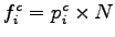
Now the computed frequency and
is shown in column (7).
Now the computed frequency  is is
 and is given in column (8).
This procedure is repeated for all the subsequent items.
It may be noted that probability of headway 9.0 is computed by one minus
probability of headway less than 9.0 and is given in column (8).
This procedure is repeated for all the subsequent items.
It may be noted that probability of headway 9.0 is computed by one minus
probability of headway less than 9.0

Table 2:
Solution using normal distribution
 |
|
 |
|
 |
 |
 |
 |
| (1) |
(2) |
(3) |
(4) |
(5) |
(6) |
(7) |
(8) |
| 1 |
0.0 |
1.0 |
0.012 |
29.21 |
0.010 |
0.038 |
92.431 |
| 2 |
1.0 |
2.0 |
0.178 |
433.25 |
0.048 |
0.111 |
269.845 |
| 3 |
2.0 |
3.0 |
0.316 |
769.14 |
0.159 |
0.211 |
513.053 |
| 4 |
3.0 |
4.0 |
0.218 |
530.61 |
0.369 |
0.261 |
635.560 |
| 5 |
4.0 |
5.0 |
0.108 |
262.87 |
0.631 |
0.211 |
513.053 |
| 6 |
5.0 |
6.0 |
0.055 |
133.87 |
0.841 |
0.111 |
269.845 |
| 7 |
6.0 |
7.0 |
0.033 |
80.32 |
0.952 |
0.038 |
92.431 |
| 8 |
7.0 |
8.0 |
0.022 |
53.55 |
0.990 |
0.008 |
20.605 |
| 9 |
8.0 |
9.0 |
0.013 |
31.64 |
0.999 |
0.001 |
2.987 |
| 10 |
9.0 |
|
0.045 |
109.53 |
1.000 |
0.010 |
24.190 |
| |
Total |
|
2434 |
|
|
|
|
|
|
| | |
|
|
|


