Module 3 : Microscopic Traffic Flow Modeling

Lecture 12 : Vehicle Arrival Models: Headway

1

2

3

4

5

6

7

8

9

10

11

12

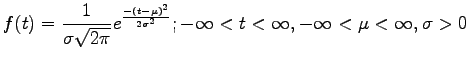
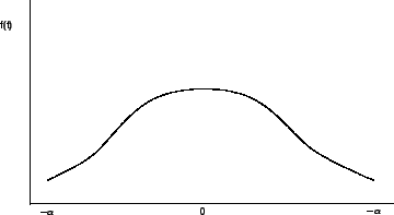
	Normal distribution The probability density function of the normal distribution is given by: $$f(t)=\frac{1}{\sigma \sqrt{2\pi}} e^{\frac{-(t-\mu)^2}{2\sigma^2}};-\infty< t <\infty, -\infty< \mu <\infty,\sigma>0$$ (1) where $\mu$ is the mean of the headway and $\sigma$ is the standard deviation of the headways. The shape of the probability density function is shown in figure 1. 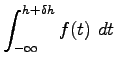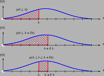Figure 1: Shape of normal distribution curve The probability that the time headway (t) less than a given time headway (h) is given by $$p(t\le h) = \int_{-\infty}^{h}f(t)~dt$$ (2) and the value of this is shown as the area under the curve in figure 2 (a) and the probability of time headway (t) less than a given time headway ( $h+\delta h$) is given by $$p(t\le h+\delta h) = \int_{-\infty}^{h+\delta h}f(t)~dt$$ (3) This is shown as the area under the curve in figure 2 (b). 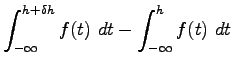Hence, the probability that the time headway lies in an interval, say $h$ and $h+\delta h$ is given by $$p(h\le t \le h+\delta h) = p(t\le h+\delta h) - p(t\le h)$$ (4) $$= \int_{-\infty}^{h+\delta h}f(t)~dt-\int_{-\infty}^{h}f(t)~dt$$ This is illustrated as the area under the curve in figure 2 (c). Figure 2: Illustration of the expression for probability that the random variable lies in an interval for normal distribution Although the probability for headway for an interval can be computed easily using equation 4, there is no closed form solution to the equation 2. Eventhough it is possible to solve the above equation by numerical integration, the computations are time consuming for regular applications. One way to overcome this difficulty is to use the standard normal distribution table which gives the solution to the equation 2 for a standard normal distribution. A standard normal distribution is normal distribution of a random variable whose mean is zero and standard deviation is one. The probability for any random variable, having a mean ($\mu$) and standard deviation ($\sigma$) can be computed by normalizing that random variable with respect to its mean and standard deviation and then use the standard normal distribution table. This is based on the concept of normalizing any normal distribution based on the assumption that if t follows normal distribution with mean $\mu$ and standard deviation $\sigma$, then $(t-\mu)/\sigma$ follows a standard normal distribution having zero mean and unit standard deviation. The normalization steps shown below. $$p[h\le t\le (h+\delta h)] = p\left[\frac{h-\mu}{\sigma}\le \frac{t-\mu}{\sigma}\le \frac{(h+\delta h)-\mu}{\sigma}\right]$$ (5) $$= p\left[t\le \frac{(h+\delta h)-\mu}{\sigma}\right] - p\left[t\le \frac{h-\mu}{\sigma}\right]$$ The first and second term in this equation be obtained from standard normal distribution table. The following example illustrates this procedure.