point

Module 3 : Microscopic Traffic Flow Modeling

Lecture 12 : Vehicle Arrival Models: Headway

Numerical Example

Given that observed mean headway is 3.5 seconds and standard distribution is 2.6 seconds, then compute the probability that the headway lies between 0 and 0.5. Assume that the minimum expected headway is 0.5 seconds.

Solution:

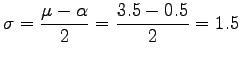
First, compute the standard deviation to be used in calculation using equation

, given that $\mu=3.5$ , $\sigma=2.6$ , and $\alpha=0.5$ . Then:

$\displaystyle \sigma=\frac{\mu-\alpha}{2}=\frac{3.5-0.5}{2}=1.5$

(1)

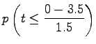
Second, compute the probability that headway less than zero.

$\displaystyle p(t<0)$	$\displaystyle \approx$	$\displaystyle p\left(t\le \frac{0-3.5}{1.5}\right)$
	$\displaystyle =$	$\displaystyle p(t\le -2.33) = 0.01$

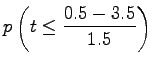
The value 0.01 is obtained from standard normal distribution table. Similarly, compute the probability that headway less than 0.5 as

$\displaystyle p(t\le 0.5)$	$\displaystyle \approx$	$\displaystyle p\left(t\le \frac{0.5-3.5}{1.5}\right)$
	$\displaystyle =$	$\displaystyle p(t<-2)$
	$\displaystyle =$	$\displaystyle 0.023$

The value 0.23 is obtained from the standard normal distribution table. Hence, the probability that headway lies between 0 and 0.5 is obtained using equation

as $p(0\le t\le 0.5)$ =