| |
| | |
|
As noted earlier, the intermediate flow is more complex since certain vehicles
will have interaction with the other vehicles and certain may not.
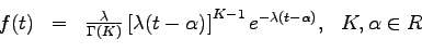
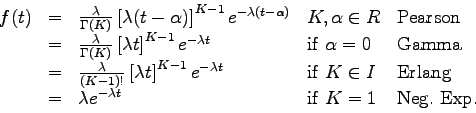
Here, Pearson Type III distribution can be used for modelling intermediate
flow.
The probability density function for the Pearson Type III distribution is given
as
 |
|
|
(1) |
where  is a parameter which is a function of is a parameter which is a function of  , ,  and and  ,
and determine the shape of the distribution.
The term is the mean of the observed headways, K is a user specified
parameter greater than 0 and is called as a shift parameter.
The ,
and determine the shape of the distribution.
The term is the mean of the observed headways, K is a user specified
parameter greater than 0 and is called as a shift parameter.
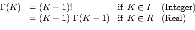
The  is the gamma function and given as is the gamma function and given as
 |
|
|
(2) |
It may also be noted that Pearson Type III is a general case of Gamma, Erlang
and Negative Exponential distribution as shown in below:
The expression for the probability that the random headway (t) is greater than
a given headway (h),  , is given as: , is given as:
and similarly
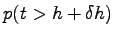 is given as: is given as:
and hence, the probability that the headway between  and and
 is
given as is
given as
It may be noted that closed form solution to equation 3 and
equation 4 is not available.
Numerical integration is also difficult due to computational requirement.
Using table as in the case of Normal
Distribution is difficult, since the table will be different for each .
A common way of solving this is by using the numerical approximation to
equation 5.
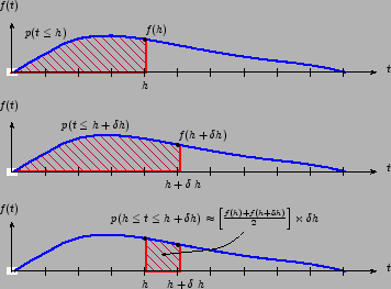
The solution to equation 5 is essentially the area under the curve defined by the probability
density function between and
.
If we assume that line joining  and and
 is linear, which is
a reasonable assumption if is linear, which is
a reasonable assumption if  is small, than the are under the curve can be found out by the following
approximate expression: is small, than the are under the curve can be found out by the following
approximate expression:
This concept is illustrated in figure 1
Figure 1:
Illustration of the expression for probability that the random
variable lies in an interval for Person Type III distribution
 |
- Input required: the mean () and the standard deviation (
 ) of
the headways. ) of
the headways.
- Set the minimum expected headway (). Say, for example, 0.5. It
means that the
 . .
- Compute the shape factor using the mean () the standard deviation
() and the minimum expected headway ()
- Compute the term flow rate () as
Note that if  and and  , then , then
 which is the
flow rate. which is the
flow rate.
- Compute gamma function value for as:
 |
(7) |
Although the closed form solution of  is available, it is difficult
to compute.
Hence, it can be obtained from gamma table.
For, example: is available, it is difficult
to compute.
Hence, it can be obtained from gamma table.
For, example:
Note that the value of
 is obtained from gamma table for is obtained from gamma table for
 which is given for which is given for
 . .
- Using equation 1 solve for by setting
 where
h is the lower value of the range and
by setting where
h is the lower value of the range and
by setting
 where
where
 is the upper value of the headway range.
Compute the probability that headway lies between the interval of and
using equation 6. is the upper value of the headway range.
Compute the probability that headway lies between the interval of and
using equation 6.
The Gamma function can be evaluated by the following approximate expression also:
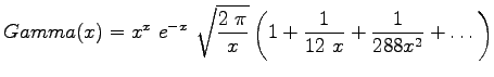 |
(8) |
|
|
| | |
|
|
|

![$\displaystyle \left[ \frac{f(h)+f(h+\delta h)}{2}
\right]\times \delta h$](img24.png)

