| |
| | |
|
The low flow traffic can be modeled using the negative exponential
distribution.
First, some basics of negative exponential distribution is presented.
The probability density function  of any distribution has the following
two important properties: First, of any distribution has the following
two important properties: First,
where  is the random variable.
This means that the total probability defined by the probability density function
is one. Second: is the random variable.
This means that the total probability defined by the probability density function
is one. Second:
![$\displaystyle p[a \le t\le b]=\int_{a}^{b}f(t)~dt$](img7.png) |
(2) |
This gives an expression for the probability that the random variable takes
a value with in an interval, which is essentially the area under the probability
density function curve.
The probability density function of negative exponential distribution is given
as:
 |
(3) |
where  is a parameter that determines the shape of the distribution
often called as the shape parameter.
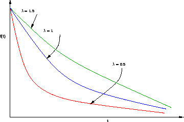
The shape of the negative exponential distribution for various values of
(0.5, 1, 1.5) is shown in figure 1. is a parameter that determines the shape of the distribution
often called as the shape parameter.
The shape of the negative exponential distribution for various values of
(0.5, 1, 1.5) is shown in figure 1.
Figure 1:
Shape of the Negative exponential distribution for various values of
 |
The probability that the random variable is greater than or equal to zero
can be derived as follow,
The probability that the random variable is greater than a specific value
 is given as is given as
Unlike many other distributions, one of the key advantages of the negative
exponential distribution is the existence of a closed form solution to the
probability density function as seen above.
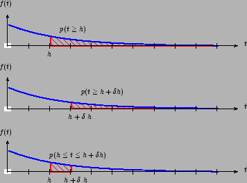
The probability that the random variable lies between an interval is given
as:
This is illustrated in figure 2.
Figure 2:
Evaluation of negative exponential distribution for an interval
 |
The negative exponential distribution is closely related to the Poisson
distribution which is a discrete distribution.
The probability density function of Poisson distribution is given as:
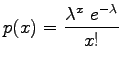 |
(7) |
where,  is the probability of is the probability of  events (vehicle arrivals) in some time
interval (),
and is the expected (mean) arrival rate in that interval.
If the mean flow rate is events (vehicle arrivals) in some time
interval (),
and is the expected (mean) arrival rate in that interval.
If the mean flow rate is  vehicles per hour, then vehicles per hour, then
 vehicles per second.
Now, the probability that zero vehicle arrive in an interval , denoted as
vehicles per second.
Now, the probability that zero vehicle arrive in an interval , denoted as
 , will be same as the probability that the headway (inter arrival time)
greater than or equal to .
Therefore, , will be same as the probability that the headway (inter arrival time)
greater than or equal to .
Therefore,
Here, is defined as average number of vehicles arriving in time .
If the flow rate is vehicles per hour, then,
 |
(8) |
Since mean flow rate is inverse of mean headway, an alternate way of
representing the probability density function of negative exponential
distribution is given as
 |
(9) |
where
 or or
 .
Here, .
Here,  is the mean headway in seconds which is again the inverse of flow
rate.
Using equation 6 and equation 5 the probability
that headway between any interval and flow rate can be computed.
The next example illustrates how a negative exponential distribution can be
fitted to an observed headway frequency distribution. is the mean headway in seconds which is again the inverse of flow
rate.
Using equation 6 and equation 5 the probability
that headway between any interval and flow rate can be computed.
The next example illustrates how a negative exponential distribution can be
fitted to an observed headway frequency distribution.
|
|
| | |
|
|
|


![$\displaystyle 1-\lambda \left[\frac{e^{-\lambda t}}{-\lambda}\right]^h_0$](img21.png)
