| |
| | |
|
Common descriptive statistics may be computed from the data in the frequency
distribution table or determined graphically from the frequency and cumulative
frequency distribution curves.
These statistics are used to describe two important characteristics of the
distribution:
Measure which helps to describe the approximate middle or center of the
distribution.
Measures of central tendency include the average or mean speed, the median
speed, the modal speed, and the pace.
Figure 1:
Frequency and Cumulative Frequency Distribution curve
|
|
The arithmetic (or harmonic) average speed is the most frequently used speed
statistics.
It is the measure of central tendency of the data. Mean calculated gives two
kinds of mean speeds.
 |
(1) |
where,  is the mean or average speed, is the mean or average speed,  is the individual speed of the is the individual speed of the
 vehicle, vehicle,  is the frequency of speed, and n is the total no of
vehicle observed (sample size).
Time mean Speed If data collected at a point over a period of time,
e.g. by radar meter or stopwatch, produce speed distribution over time, so the
mean of speed is time mean speed.
Space mean Speed If data obtained over a stretch (section) of road
almost instantaneously, aerial photography or enoscope, result in speed
distribution in space and mean is space mean speed.
Distribution over space and time are not same.
Time mean speed is higher than the space mean speed.
The spot speed sample at one end taken over a finite period of time will tend
to include some fast vehicles which had not yet entered the section at the
start of the survey, but will exclude some of the slower vehicles.
The relationship between the two mean speeds is expressed by: is the frequency of speed, and n is the total no of
vehicle observed (sample size).
Time mean Speed If data collected at a point over a period of time,
e.g. by radar meter or stopwatch, produce speed distribution over time, so the
mean of speed is time mean speed.
Space mean Speed If data obtained over a stretch (section) of road
almost instantaneously, aerial photography or enoscope, result in speed
distribution in space and mean is space mean speed.
Distribution over space and time are not same.
Time mean speed is higher than the space mean speed.
The spot speed sample at one end taken over a finite period of time will tend
to include some fast vehicles which had not yet entered the section at the
start of the survey, but will exclude some of the slower vehicles.
The relationship between the two mean speeds is expressed by:
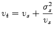 |
(2) |
where, and  are the time mean speed and space mean speed
respectively.
And are the time mean speed and space mean speed
respectively.
And  is the standard deviation of distribution space.
The median speed is defined as the speed that divides the distribution in to
equal parts (i.e., there are as many observations of speeds higher than the
median as there are lower than the median).
It is a positional value and is not affected by the absolute value of extreme
observations. By definition, the median equally divides the distribution.
Therefore, 50% of all observed speeds should be less than the median.
In the cumulative frequency curve, the 50th percentile speed is the median of
the speed distribution.
Median Speed = v50
The pace is a traffic engineering measure not commonly used for other
statistical analyses.
It is defined as the 10Km/h increment in speed in which the highest percentage
of drivers is observed.
It is also found graphically using the frequency distribution curve. As shown
in fig 6.5.
The pace is found as follows: A 10 Km/h template is scaled from the horizontal
axis.
Keeping this template horizontal, place an end on the lower left side of the
curve and move slowly along the curve.
When the right side of the template intersects the right side of the curve,
the pace has been located.
This procedure identifies the 10 Km/h increments that intersect the peak of
the curve; this contains the most area and, therefore, the highest percentage
of vehicles.
The mode is defined as the single value of speed that is most likely to occur.
As no discrete values were recorded, the modal speed is also determined
graphically from the frequency distribution curve.
A vertical line is dropped from the peak of the curve, with the result found on
the horizontal axis. is the standard deviation of distribution space.
The median speed is defined as the speed that divides the distribution in to
equal parts (i.e., there are as many observations of speeds higher than the
median as there are lower than the median).
It is a positional value and is not affected by the absolute value of extreme
observations. By definition, the median equally divides the distribution.
Therefore, 50% of all observed speeds should be less than the median.
In the cumulative frequency curve, the 50th percentile speed is the median of
the speed distribution.
Median Speed = v50
The pace is a traffic engineering measure not commonly used for other
statistical analyses.
It is defined as the 10Km/h increment in speed in which the highest percentage
of drivers is observed.
It is also found graphically using the frequency distribution curve. As shown
in fig 6.5.
The pace is found as follows: A 10 Km/h template is scaled from the horizontal
axis.
Keeping this template horizontal, place an end on the lower left side of the
curve and move slowly along the curve.
When the right side of the template intersects the right side of the curve,
the pace has been located.
This procedure identifies the 10 Km/h increments that intersect the peak of
the curve; this contains the most area and, therefore, the highest percentage
of vehicles.
The mode is defined as the single value of speed that is most likely to occur.
As no discrete values were recorded, the modal speed is also determined
graphically from the frequency distribution curve.
A vertical line is dropped from the peak of the curve, with the result found on
the horizontal axis.
|
|
| | |
|
|
|
![\includegraphics[height = 5cm]{qffrequencycfcurve}](img1.png)