| |
| | |
|
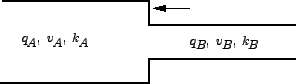
The flow of traffic along a stream can be considered similar to a fluid flow.
Consider a stream of traffic flowing with steady state conditions, i.e., all the
vehicles in the stream are moving with a constant speed, density and flow. Let
this be denoted as state A (refer figure 1.
Suddenly due to some obstructions in the stream (like an accident or traffic
block) the steady state characteristics changes and they acquire another state
of flow, say state B.
The speed, density and flow of state A is denoted as  , ,
 , and , and  , and state B as , and state B as  , ,  , and , and  respectively.
Figure 1:
Shock wave: Stream characteristics
 |
The flow-density curve is shown in figure 2.
Figure 2:
Shock wave: Flow-density curve
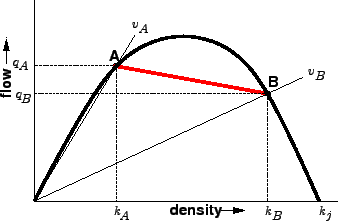 |
The speed of the vehicles at state A is given by the line
joining the origin and point A in the graph.
The time-space diagram of the traffic stream is also plotted
in figure 3.
Figure 3:
Shock wave : time-distance diagram
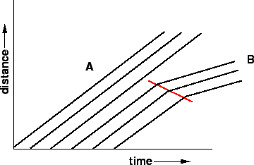 |
All the lines are having the same slope which
implies that they are moving with constant speed.
The sudden change in the characteristics of the stream leads
to the formation of a shock wave.
There will be a cascading effect of the vehicles in the
upstream direction.
Thus shock wave is basically the movement of the point that
demarcates the two stream conditions.
This is clearly marked in the figure 2.
Thus the shock waves produced at state B are propagated in
the backward direction.
The speed of the vehicles at state B is the line joining the
origin and point B of the flow-density curve.
Slope of the line AB gives the speed of the shock wave
(refer figure 2).
If speed of the shock-wave is represented as
 , then , then
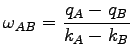 |
(1) |
The above result can be analytically solved by equating the
expressions for the number vehicles leaving the upstream and
joining the downstream of the shock wave boundary (this
assumption is true since the vehicles cannot be created or
destroyed.
Let  be the number of vehicles leaving the section A.
Then, be the number of vehicles leaving the section A.
Then,  .
The relative speed of these vehicles with respect to the
shock wave will be .
The relative speed of these vehicles with respect to the
shock wave will be
 .
Hence, .
Hence,
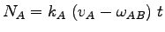 |
(2) |
Similarly, the vehicles entering the state B is given as
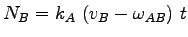 |
(3) |
Equating equations 2 and 3, and solving
for
as follows will yield to:
This will yield the following expression for the shock-wave
speed.
|
(4) |
In this case, the shock wave move against the direction of
traffic and is therefore called a backward moving shock
wave.
There are other possibilities of shock waves such as forward
moving shock waves and stationary shock waves.
The forward moving shock waves are formed when a stream with
higher density and higher flow meets a stream with
relatively lesser density and flow.
For example, when the width of the road increases suddenly,
there are chances for a forward moving shock wave.
Stationary shock waves will occur when two streams having the
same flow value but different densities meet.
|
|
| | |
|
|
|