Module 1 : Traffic Stream Characteristics

Lecture 03 : Traffic Stream Models

1

2

3

4

5

6

7

8

9

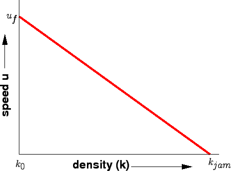
	Greenshield's macroscopic stream model Macroscopic stream models represent how the behaviour of one parameter of traffic flow changes with respect to another. Most important among them is the relation between speed and density. The first and most simple relation between them is proposed by Greenshield. Greenshield assumed a linear speed-density relationship as illustrated in figure 1 to derive the model. Figure 1: Relation between speed and density The equation for this relationship is shown below. $$v = v_f -\left[\frac{v_f}{k_j}\right].k$$ (1) where $v$ is the mean speed at density $k$, $v_f$ is the free speed and $k_j$ is the jam density. This equation ( 1) is often referred to as the Greenshield's model. It indicates that when density becomes zero, speed approaches free flow speed (ie. $v~\rightarrow ~v_f~$ when $k\rightarrow 0$). 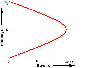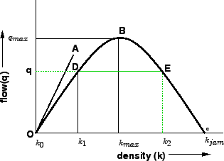Figure 2: Relation between speed and flow Once the relation between speed and flow is established, the relation with flow can be derived. This relation between flow and density is parabolic in shape and is shown in figure 3. Also, we know that $$q = k.v$$ (2) Figure 3: Relation between flow and density 1 Now substituting equation 1 in equation 2, we get $$q = v_f.k -\left [{\frac{v_f}{k_j}}\right] k^2$$ (3) Similarly we can find the relation between speed and flow. For this, put $k=\frac{q}{v}$ in equation 1 and solving, we get $$q = k_j.v -\left[{\frac{k_j}{v_f}}\right] v^2$$ (4) This relationship is again parabolic and is shown in figure 2. Once the relationship between the fundamental variables of traffic flow is established, the boundary conditions can be derived. The boundary conditions that are of interest are jam density, free-flow speed, and maximum flow. To find density at maximum flow, differentiate equation 3 with respect to $k$ and equate it to zero. ie., $$\frac{dq}{dk} =$$ 0 $$v_f-\frac{v_f}{k_j}.2k =$$ 0 $$k = \frac{k_j}{2}$$ Denoting the density corresponding to maximum flow as $k_0$, $$k_0=\frac{k_j}{2}$$ (5) Therefore, density corresponding to maximum flow is half the jam density. Once we get $k_0$, we can derive for maximum flow, $q_{max}$. Substituting equation 5 in equation 3 $$q_{max} = v_f. \frac {k_j}{2}-\frac{v_f}{k_j}. \left[{\frac{k_j}{2}}\right]^2$$ $$= v_f.\frac{k_j}{2} - v_f.\frac{k_j}{4}$$ $$= \frac{{v_f}.{k_j}}{4}$$ Thus the maximum flow is one fourth the product of free flow and jam density. Finally to get the speed at maximum flow, $v_0$, substitute equation 5 in equation 1 and solving we get, $$v_0 = v_f - \frac{v_f}{k_j}.\frac{k_j}{2}$$ $$v_0 = \frac{v_f}{2}$$ (6) Therefore, speed at maximum flow is half of the free speed.